Cobweb plots
Posted on 01 November 2017
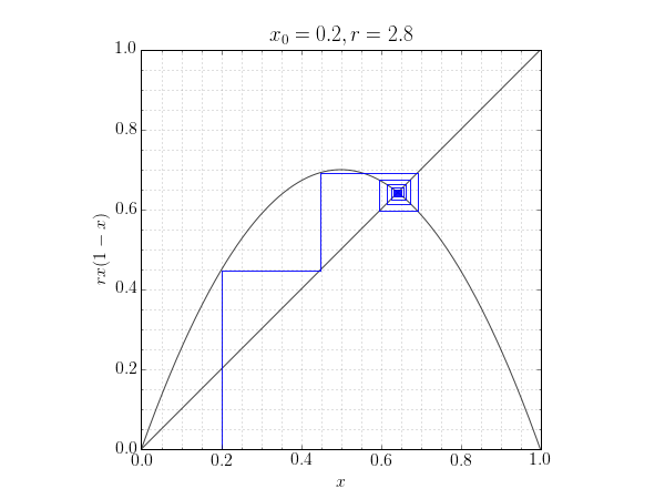
A cobweb plot is often used to visulaize the behaviour of an iterated function. That is, the sequence of values obtained from setting $x_{n+1} = f(x_n)$, starting at some value $x_0$.
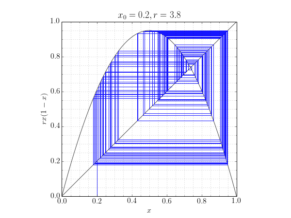
The plot can reveal stable, cyclic, or chaotic behaviour as convergence to a point, a repeating rectangle or by filling the plane with non-repeating line segments respectively.
The code below generates a cobweb plot for the logistic map: $f(x) = rx(1-x)$. With a chosen starting value of $x_0=0.5$, both stable and chaotic behaviour is observed for different values of $r$.
import numpy as np
from matplotlib import rc
import matplotlib.pyplot as plt

# Use LaTeX throughout the figure for consistency
rc('font', **{'family': 'serif', 'serif': ['Computer Modern'], 'size': 16})
rc('text', usetex=True)
# Figure dpi
dpi = 72

def plot_cobweb(f, r, x0, nmax=40):
    """Make a cobweb plot.

    Plot y = f(x; r) and y = x for 0 <= x <= 1, and illustrate the behaviour of
    iterating x = f(x) starting at x = x0. r is a parameter to the function.

    """
    x = np.linspace(0, 1, 500)
    fig = plt.figure(figsize=(600/dpi, 450/dpi), dpi=dpi)
    ax = fig.add_subplot(111)

    # Plot y = f(x) and y = x
    ax.plot(x, f(x, r), c='#444444', lw=2)
    ax.plot(x, x, c='#444444', lw=2)

    # Iterate x = f(x) for nmax steps, starting at (x0, 0).
    px, py = np.empty((2,nmax+1,2))
    px[0], py[0] = x0, 0
    for n in range(1, nmax, 2):
        px[n] = px[n-1]
        py[n] = f(px[n-1], r)
        px[n+1] = py[n]
        py[n+1] = py[n]

    # Plot the path traced out by the iteration.
    ax.plot(px, py, c='b', alpha=0.7)

    # Annotate and tidy the plot.
    ax.minorticks_on()
    ax.grid(which='minor', alpha=0.5)
    ax.grid(which='major', alpha=0.5)
    ax.set_aspect('equal')
    ax.set_xlabel('$x$')
    ax.set_ylabel(f.latex_label)
    ax.set_title('$x_0 = {:.1}, r = {:.2}$'.format(x0, r))

    plt.savefig('cobweb_{:.1}_{:.2}.png'.format(x0, r), dpi=dpi)

class AnnotatedFunction:
    """A small class representing a mathematical function.

    This class is callable so it acts like a Python function, but it also
    defines a string giving its latex representation.

    """

    def __init__(self, func, latex_label):
        self.func = func
        self.latex_label = latex_label

    def __call__(self, *args, **kwargs):
        return self.func(*args, **kwargs)

# The logistic map, f(x) = rx(1-x).
func = AnnotatedFunction(lambda x,r: r*x*(1-x), r'$rx(1-x)$')

plot_cobweb(func, 2.8, 0.2)
plot_cobweb(func, 3.8, 0.2, 200)