A superellipse (also called a Lamé curve) is the curve described by the equation
\[\left|\frac{x}{a}\right|^p + \left|\frac{y}{b}\right|^p = 1\]
For \(n=2\), this is the equation of an ordinary ellipse and for \(a=b=1\) that ellipse is a circle. The corresponding curve for \(p=4\) is sometimes called a squircle.
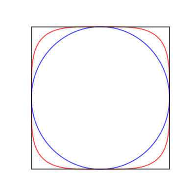
As \(p \rightarrow \infty\), the curve approaches the form of a square. The code below plots a few superellipses for \(2 \le p \le 25\) and indicates how the area approaches unity as \(p\) gets larger. It turns out to be easier to use the parametric representation of the superellipse:
\[\begin{align*}
x(t) &= |\cos t|^{2/n}a\cdot\mathrm{sgn}(\cos t)\\
y(t) &= |\sin t|^{2/n}b\cdot\mathrm{sgn}(\sin t)
\end{align*}\]
for \(0\le t \le 2\pi\).
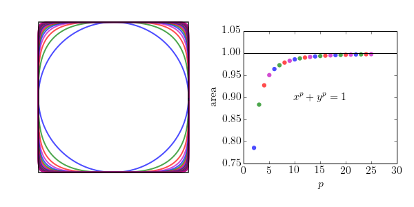
The area of a super ellipse may be written in terms of the gamma function as:
\[A = 4ab\frac{\left[\Gamma\left(1+\frac{1}{n}\right)\right]^2}{\Gamma\left(1+\frac{2}{n}\right)}\]
import numpy as np
from scipy.special import gamma
from matplotlib import rc
import matplotlib.pyplot as plt
from itertools import cycle

# Use LaTeX throughout the figure for consistency
rc('font', **{'family': 'serif', 'serif': ['Computer Modern'], 'size': 16})
rc('text', usetex=True)

# Set up the figure.
dpi = 72
fig, (ax1, ax2) = plt.subplots(1, 2, figsize=(600/dpi, 300/dpi), dpi=dpi)

# These are the colours we'll cycle through
colour_cycle = cycle(['b', 'g', 'r', 'm'])

# The parameter t in the parametric description of the superellipse
t = np.linspace(0, 2*np.pi, 500)

# Build an array of values of p up to pmax and assign the corresponding colours
pmax = 26
pvals = np.arange(2, pmax, dtype=int)
colour = [next(colour_cycle) for i in range(pvals.shape[0])]

# All the superellipses will have these plot arguments in common
kwargs = {'lw': 2, 'alpha': 0.7}

# Plot the superellipses
for i,p in enumerate(pvals):
    c, s = np.cos(t), np.sin(t)
    x = np.abs(c)**(2/p) * np.sign(c)
    y = np.abs(s)**(2/p) * np.sign(s)
    ax1.plot(x, y, c=colour[i], **kwargs)

# Draw a unit square.
ax1.plot([-1,-1,1,1,-1],[-1,1,1,-1,-1], c='k', **kwargs)
# The x- and y-axes must be scaled the same for circles to look circular.
ax1.axis('equal')
ax1.axis('off')

# Plot the superellipses' areas as a function of p.
ax2.scatter(pvals, gamma(1 + 1/pvals)**2 / gamma(1 + 2/pvals), c=colour,
            lw=0, alpha=0.7, s=40)
# Label, annotate and tidy this plot
ax2.set_xlabel(r'$p$')
ax2.set_ylabel('area')
ax2.annotate(s=r'$x^p + y^p = 1$', xy=(0.5, 0.5), xycoords='axes fraction',
             ha='center', va='center')

ymin, ymax = ax2.get_ylim()
ax2.set_aspect(pmax / (ymax-ymin))
ax2.axhline(1.0, lw=1, c='k')

fig.tight_layout()
plt.savefig('superellipse.png', dpi=dpi)