Processing UK Ordnance Survey terrain data
Posted on 10 October 2019
The UK's Ordnance Survey mapping agency now makes its 50 m resolution elevation data freely-available through its online OpenData download service. This article uses Python, NumPy and Matplotlib to process and visualize these data without using a specialized GIS library.
First create a directory, such as terrain50/, and within it create a second directory, data/. From the OpenData website select ASCII Grid and GML (Grid) and download the archive and unzip it to terr50_gagg_gb/ inside data/. This unzipped archive contains further zipped data files containing .asc files named XX##.asc where XX is a two-letter code identifying each 100 km × 100 km grid sq of the OS map and ## identifies the 10 km × 10 km grid squares within this larger square. For more on the OS grid system, see this Beginner's Guide.
From within terrain50/data/, unzip all the files with
find . -name "*.zip" -exec unzip '{}' ';'
(On a Mac / Unix / Linux system; on Windows do ... something else). You can now delete the archive, terr50_gagg_gb/ directory and any file that doesn't end in .asc to save space.
It will be convenient to extract all the elevation data into a single NumPy array, saved in the platform-independent binary .npy:
import os
import glob
import numpy as np
import matplotlib.pyplot as plt

DATA_DIR = 'data'
asc_files = glob.glob(os.path.join(DATA_DIR, '*.asc'))

def read_asc_file(filename):
    """Read the .asc file filename and return its data."""

    with open(filename) as fi:
        # Skip the first two header lines
        fi.readline(); fi.readline()
        # This are the lower left corner coordinates
        xll = int(fi.readline().split()[1])
        yll = int(fi.readline().split()[1])
        # Skip the next line
        fi.readline()

        # There may be an extra line indicating the value used to represent
        # missing data. If there isn't we'll need to rewind to the start of
        # this line before we start reading data with np.genfromtxt.
        pos = fi.tell()
        line = fi.readline()
        nan_val = None
        if line.startswith('nodata_value'):
            nan_val = float(line.split()[1])
        else:
            fi.seek(pos)

        sq = np.genfromtxt(fi, delimiter=' ')
        if nan_val is not None:
            # If we care to, here's where we would replace the default value
            # representing missing data with np.nan or something else.
            pass

    # Return the indexes into arr for this square and the data itself.
    return xll//50, yll//50, sq

# The OS data covers 700 km x 1,300 km at a resolution of 50 m.
nx, ny = 700000 // 50, 1300000 // 50
# We don't need double precision; float32 will be fine.
arr = np.zeros((ny, nx), dtype='float32')

# If we only care about certain 100 km x 100 km squares specify them here: e.g.
squares = 'HO', 'HP', 'SV', 'TM'
ftu = [f'data/{s}' for s in squares]

nfiles = len(asc_files)
for i, asc_file in enumerate(asc_files):
    # Uncomment this line if we only want the squares specified above
    #if not any([asc_file.startswith(f) for f in ftu]):
    #    continue

    # Progress report.
    print(f'{i+1}/{nfiles}:', asc_file)
    # Get the square and update arr in the correct orientation.
    xll, yll, sq = read_asc_file(asc_file)
    arr[yll:yll+200, xll:xll+200] = sq[::-1,:]

print('Saving terrain...')
np.save('terr-50.npy', arr)

# Comment out these lines if you don't need to check the data and/or you're
# low on memory.
plt.imshow(arr, origin='lower')
plt.show()
To bin the data to a lower resolution, we can read in terr-50.npy and use the same NumPy methods demonstrated in this previous post.
import numpy as np
import matplotlib.pyplot as plt

# Binning factors in x- and y-directions
BX, BY = 40, 200

# Load the terrain array; with regret, chop off the Orkneys and Shetland.
arr = np.load('terr-50.npy')[:22000,:]
ny, nx = arr.shape

def rebin(arr, new_shape):
    """Rebin 2D array arr to shape new_shape by averaging."""

    shape = (new_shape[0], arr.shape[0] // new_shape[0],
             new_shape[1], arr.shape[1] // new_shape[1])
    return arr.reshape(shape).mean(-1).mean(1)

arr = rebin(arr, (ny // BY, nx // BX))
np.save('terr-50-binned.npy', arr)

plt.imshow(arr, origin='lower')
plt.show()
The resulting file is available here: terr-50-binned.npy and is 151 kB in size instead of 1.4 GB.
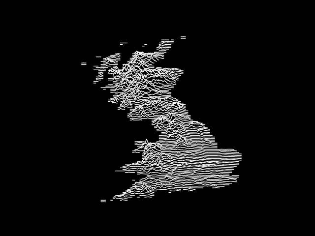
Finally, to create the above image:
import numpy as np
import matplotlib.pyplot as plt

# Load the binned terrain array.
arr = np.load('terr-50-binned.npy')
# Set the sea to NaN
arr[arr==0] = np.nan
ny, nx = arr.shape

fig = plt.figure(facecolor='k')
ax = fig.add_subplot(facecolor='k')
x = np.arange(nx)

# DROW controls the spacing between rows: higher will reduce the vertical
# resolution.
DROW = 150

# Draw the terrain in a series of white lines from left to right:
for i, row in enumerate(arr):
    offset = i * DROW
    zorder = (ny*DROW - offset+1)*2
    ax.plot(x, row+offset, 'w', zorder=zorder, lw=1)
    ax.fill_between(x, row+offset, offset, facecolor='k', lw=0,
                    zorder=zorder-1)

# Tweak the appearance to get the aspect ratio right and to remove the axes.
sc = nx/ny
ax.set_aspect(sc/DROW)
ax.axis('off')

# We need to specify the figure facecolour again in savefig.
plt.savefig('os-uk.png', facecolor=fig.get_facecolor(), edgecolor='none')
plt.show()