The standard way to bin a large array to a smaller one by averaging is to reshape it into a higher dimension and then take the means over the appropriate new axes. The following function does this, assuming that each dimension of the new shape is a factor of the corresponding dimension in the old one.

def rebin(arr, new_shape):
    shape = (new_shape[0], arr.shape[0] // new_shape[0],
             new_shape[1], arr.shape[1] // new_shape[1])
    return arr.reshape(shape).mean(-1).mean(1)

To see how this works, consider reshaping a $4 \times 6$ array to become $2 \times 3$:

In [x]: arr = np.arange(24).reshape((4,6))
In [x]: arr
Out[x]: 
array([[ 0,  1,  2,  3,  4,  5],
       [ 6,  7,  8,  9, 10, 11],
       [12, 13, 14, 15, 16, 17],
       [18, 19, 20, 21, 22, 23]])

We reshape from (4, 6) to (2, 4//2, 3, 6//3) = (2, 2, 3, 2):

In [x]: arr.reshape(2, 4//2, 3, 6//3)
Out[x]: 
array([[[[ 0,  1],
         [ 2,  3],
         [ 4,  5]],

        [[ 6,  7],
         [ 8,  9],
         [10, 11]]],


       [[[12, 13],
         [14, 15],
         [16, 17]],

        [[18, 19],
         [20, 21],
         [22, 23]]]])

This has grouped entries so that each row has become a $3 \times 2$ subarray and these subarrays are arranged as entries in the first $2 \times 2$ dimensions of the new 4D array. Now consider averaging over the last dimension (indexed with -1):

In [x]: arr.reshape(2, 2, 3, 2).mean(-1)
Out[x]: 
array([[[  0.5,   2.5,   4.5],
        [  6.5,   8.5,  10.5]],

       [[ 12.5,  14.5,  16.5],
        [ 18.5,  20.5,  22.5]]])

This has averaged entries along each row to leave an array of shape (2,2,3) (for example, the first entry is the average of 0 and 1, which is 0.5). Now, averaging over the second dimension of this array (indexed with 1) corresponding to columns of the original array:

In [x]: arr.reshape(2, 2, 3, 2).mean(-1).mean(1)
Out[x]: 
array([[  3.5,   5.5,   7.5],
       [ 15.5,  17.5,  19.5]])

This is the $2\times 3$ binned array that we wanted.

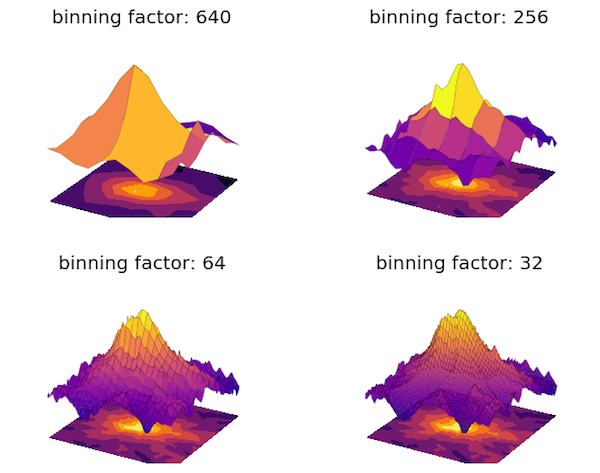
Here is an illustration of the technique, based on USGS elevation data for the vicinity of Mt Ranier, which can be obtained from their download service.

import os
from osgeo import gdal
import numpy as np
import matplotlib.pyplot as plt
from matplotlib import cm
from mpl_toolkits.mplot3d import Axes3D

imgdir = '/Users/christian/temp/mt-ranier'

# Mt Ranier spans two IMG files in the USGS data set.
imgnameW = 'ned19_n47x00_w122x00_wa_mounttrainier_2008'
imgnameE = 'ned19_n47x00_w121x75_wa_mounttrainier_2008'

def get_elev_arr(imgname):
    """Read in the elevation data as a NumPy array."""

    imgfile = os.path.join(imgdir, imgname, imgname+'.img')
    print(imgfile)
    geo = gdal.Open(imgfile)
    arr = geo.ReadAsArray()
    # invalid or missing data is indicated by a large negative value, so
    # replace these entries with NaN.
    arr[arr<0] = np.nan
    return arr

# stack the East and West arrays next to each other to give elevation across
# the entire area.
elev = np.hstack((get_elev_arr(imgnameW), get_elev_arr(imgnameE)))

# The latitude and longitude bounds of the elevation array
N, S = 47.000185185185195, 46.749814814814826
E, W = -121.49981481481484, -122.00018518518522

# The centre of the mountain
clat, clong = 46.88, -121.70

# Extract the region in a square centred on the Mt Ranier
Ny, Nx = elev.shape
icx, icy = int((N-clat)/(N-S) * Nx), int((W-clong)/(W-E) * Ny)
Dpx = 3200
ix1, iy1, ix2, iy2 = icx-Dpx, icy-Dpx, icx+Dpx, icy+Dpx
nx, ny = ix2-ix1, iy2-iy1
elev = elev[iy1:iy2,ix1:ix2]

def rebin(arr, new_shape):
    """Rebin 2D array arr to shape new_shape by averaging."""
    shape = (new_shape[0], arr.shape[0] // new_shape[0],
             new_shape[1], arr.shape[1] // new_shape[1])
    return arr.reshape(shape).mean(-1).mean(1)

# Create four surface subplots with different binnings
fig, axes = plt.subplots(nrows=2, ncols=2, subplot_kw={'projection': '3d'})
binfacs = (640, 256, 64, 32)
for i, binfac in enumerate(binfacs):
    ax = axes[i // 2, i % 2]
    bnx, bny = nx//binfac, ny//binfac
    X, Y = np.linspace(1,bnx,bnx), np.linspace(1,bny,bny)
    X, Y = np.meshgrid(Y, X)
    binned_elev = rebin(elev, (bny, bnx))
    ax.plot_surface(X, Y, binned_elev, rstride=4, cstride=4, linewidth=0.1,
                antialiased=True, cmap=cm.plasma)

    cset = ax.contourf(X, Y, binned_elev, zdir='z', offset=0, cmap=cm.inferno)
    ax.set_axis_off()
    ax.dist=12
plt.savefig('ranier-rebinned.png')
plt.show()