Posted by: christian on 4 Mar 2024
The Kapitza pendulum is an inverted pendulum that can balance stably when driven by an oscillating vertical displacement. As with previous posts, the position of the pendulum bob with time can be described using Lagrangian mechanics. In a coordinate system with the pendulum anchor driven vertically around (0,0) and the y-axis pointing up, the components of the bob position and velocity as a function of time are:
\begin{align*} x &= l\sin\theta\\ y &= -l\cos\theta - a \cos\omega t\\ \dot{x} &= -l\dot{\theta}\cos\theta\\ \dot{y} &= l\dot{\theta}\sin\theta - a\omega\sin\omega t \end{align*}
where $l$ is the length of the (rigid) pendulum rod and $\theta$ is its angular displacement anticlockwise from the downwards vertical. The kinetic energy, $T = \tfrac{1}{2}m(\dot{x}^2 + \dot{y}^2)$, and potential energy, $V = mgy$, are then as follows:
\begin{align*} T &= \frac{m}{2}\left[ l^2\dot{\theta}^2\cos^2\theta + l^2\dot{\theta}^2\sin^2\theta + a^2\omega^2\sin^2\omega t - 2l\dot{\theta}a\omega\sin\theta\sin\omega t\right]\\ &= \frac{m}{2}\left[ l^2\dot{\theta}^2 + a^2\omega^2\sin^2\omega t - 2l\dot{\theta}a\omega\sin\theta\sin\omega t\right],\\ V &= mg\left[l\cos\theta + a\cos\omega t\right]. \end{align*}
and give the Lagrangian, $\mathcal{L} = T - V$. The Euler-Lagrange equation is then:
\begin{align*} & \frac{\mathrm{d}}{\mathrm{d}t} \frac{\partial\mathcal{L}}{\partial\dot{\theta}} = \frac{\partial\mathcal{L}}{\partial\theta}\\ \Rightarrow \; & l^2\ddot{\theta} - la\omega(\omega\sin\theta\cos\omega t + \dot{\theta}\cos\theta\sin\omega t) = -la\omega\dot{\theta}\cos\theta\sin\omega t - gl\sin\theta. \end{align*}
This expression can be readily rearranged to give the following equation of motion:
$$ \ddot{\theta} = \frac{a\omega^2}{l}\sin\theta\cos\omega t - \frac{g}{l}\sin\theta. $$
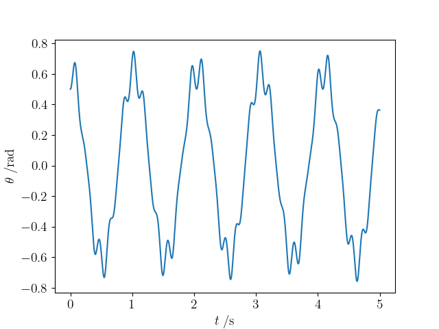
The code below uses the scipy.integrate.solve_ivp method to integrate the above differential equation and plots the angular displacement as a function of time as well as giving the frames of an animation of the behaviour of the Kapitza pendulum.
(This animation has been slowed down to better show the two frequencies of motion.)
from pathlib import Path
import numpy as np
from scipy.integrate import solve_ivp
import matplotlib.pyplot as plt
from matplotlib import rc
rc('font', **{'family': 'serif', 'serif': ['Computer Modern'], 'size': 14})
rc('text', usetex=True)

FRAMES_DIR = Path('frames')

m, L = 1, 1
a = 0.2
w = 40
g = 9.81

def deriv(t, y, L, a, w):
    """Return the first derivatives of y = theta, dtheta/dt."""
    theta, thetadot = y

    wt = w * t
    cwt = np.cos(wt)
    cth, sth = np.cos(theta), np.sin(theta)

    thetadotdot = a * w**2 / L * sth * cwt - g / L * sth
    return thetadot, thetadotdot

# Maximum time, time point spacings and the time grid (all in s).
tmax, dt = 5, 1/w/10
t = np.arange(0, tmax, dt)
# Initial conditions: theta, dtheta/dt.
y0 = [0.5, 0]    # 3 is not quite pi: the bob points not quite straight up.

tspan = (0, tmax)
sol = solve_ivp(deriv, tspan, y0, t_eval=t, args=(L, a, w))
theta = sol.y[0]
plt.plot(sol.t, theta)
plt.xlabel('$t\;/\mathrm{s}$')
plt.ylabel(r'$\theta\;/\mathrm{rad}$')
plt.show()
plt.savefig('kapitza.png')
import sys; sys.exit()

# Convert to Cartesian coordinates of the two bob positions.
x = L * np.sin(theta)
y = -L * np.cos(theta) - a * np.cos(w * sol.t)

# Plotted bob circle radius
r = 0.05

def make_plot(i):
    """
    Plot and save an image of the inverted pendulum configuration for time
    point i.

    """

    y0 = -a * np.cos(w*sol.t[i])
    ax.plot([0, x[i]], [y0, y[i]], c='k', lw=2)
    # Circles representing the anchor point of rod 1 and the bobs
    c0 = plt.Circle((0, y0), r/2, fc='k', zorder=10)
    c1 = plt.Circle((x[i], y[i]), r, fc='r', ec='r', zorder=10)
    ax.add_patch(c0)
    ax.add_patch(c1)

    # Centre the image on the fixed anchor point, and ensure the axes are equal
    ax.set_xlim(-L-r, L+r)
    ax.set_ylim(-L-a-r, L+a+r)
    ax.set_aspect('equal', adjustable='box')
    plt.axis('off')
    filename = FRAMES_DIR / f"_img{i//di:04d}.png"
    plt.savefig(filename, dpi=72)
    # Clear the Axes ready for the next image.
    plt.cla()


# Make an image every di time points.
di = 4
# This figure size (inches) and dpi give an image of 600x450 pixels.
fig = plt.figure(figsize=(8.33333333, 6.25), dpi=72)
ax = fig.add_subplot(111)

for i in range(0, t.size, di):
    print(i // di, '/', t.size // di)
    make_plot(i)
Comments
Comments are pre-moderated. Please be patient and your comment will appear soon.
There are currently no comments
New Comment