The harmonically-driven pendulum
Posted on 25 July 2017
For the purposes of this article, the harmonically-driven pendulum is one whose anchor point moves in time according to $x_0(t) = A\cos\omega t$. As with previous posts, the position of the pendulum bob with time can be described using Lagrangian mechanics. In a coordinate system with the pendulum anchor initially at $(0,0)$ and the $y$-axis pointing up, the components of the bob position and velocity as a function of time are:
$$ \begin{align*} x &= l\sin\theta + A\cos\omega t& \dot{x} &= l\dot{\theta}\cos\theta - A\omega\sin\omega t\\ y &= -l\cos\theta & \dot{y} &= l\dot{\theta}\sin\theta \end{align*} $$
The kinetic energy, $T = \tfrac{1}{2}m(\dot{x}^2 + \dot{y}^2)$, and potential energy, $V = mgy$ then give the Lagrangian, $\mathcal{L} = T - V$ as
$$ \mathcal{L} = T - V = \tfrac{1}{2}m(l^2\dot{\theta}^2 + A^2\omega^2\sin^2\omega t - 2A\omega l \dot{\theta}\sin\omega t\cos\theta) + mgl\cos\theta, $$
and the Euler-Lagrange equation leads to the following equation of motion:
$$ \ddot{\theta} = \frac{A\omega^2}{l}\cos\omega t - \frac{g}{l}\sin\theta. $$ This equation cannot be solved analytically, but in the limit of small $\theta$ it reduces to the second-order non-homogeneous differential equation:
$$ \ddot{\theta} \approx \frac{A\omega^2}{l}\cos\omega t - \frac{g}{l}\theta $$
which may be solved by standard methods to give
$$ \theta_\mathrm{approx} = \frac{A\omega^2}{l(\omega_0^2-\omega^2)}(\cos\omega t - \cos\omega_0 t), $$
for the simplest initial conditions, $\theta(0) = \dot{\theta}(0) = 0$, where $\omega_0 = \sqrt{g/l}$ is the pendulum's "natural" frequency.
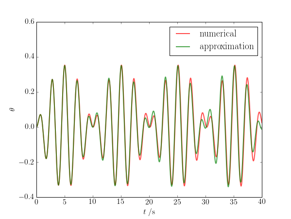
Here is a plot of both $\theta(t)$ and $\theta_\mathrm{approx}(t)$ for a small driving amplitude, $A$. Because of resonance (when $\omega \approx \omega_0$), even a small $A$ is not guaranteed to keep $\theta$ small enough for the approximate formula to hold indefinitely.
Here is the Python code. As before, the frames of the animation are placed in a directory frames/.
import numpy as np
from scipy.integrate import odeint
import matplotlib.pyplot as plt
from matplotlib.patches import Circle

# Pendulum rod length (m), drive frequency (s-1), amplitude (m), mass (kg)
L, w, A, m = 1, 2.5, 0.1, 1
# The gravitational acceleration (m.s-2).
g = 9.81

def deriv(y, t, L, w, A, m):
    """Return the first derivatives of y = theta, z1, L, z2."""
    theta, thetadot = y

    dtheta_dt = thetadot
    dthetadot_dt = (A * w**2 / L * np.cos(w*t) * np.cos(theta) -
                   g * np.sin(theta))
    return dtheta_dt, dthetadot_dt

# Maximum time, time point spacings and the time grid (all in s).
tmax, dt = 40, 0.01
t = np.arange(0, tmax+dt, dt)
# Initial conditions: theta, dtheta/dt
y0 = [0, 0]

# Do the numerical integration of the equations of motion
y = odeint(deriv, y0, t, args=(L, w, A, m))
# Unpack theta and thetadot as a function of time
theta, thetadot = y[:,0], y[:,1]

# Convert to Cartesian coordinates of the two bob positions.
x = L * np.sin(theta)
y = -L * np.cos(theta)

# Plotted bob circle radius
r = 0.05
# Plot a trail of the m2 bob's position for the last trail_secs seconds.
trail_secs = 1
# This corresponds to max_trail time points.
max_trail = int(trail_secs / dt)

def make_plot(i):
    """
    Plot and save an image of the spring pendulum configuration for time
    point i.

    """

    x0 = A * np.cos(w * t[i])
    plt.plot([x0, x0+x[i]], [0, y[i]])
    # Circles representing the anchor point of rod 1 and the bobs
    c0 = Circle((x0, 0), r/2, fc='k', zorder=10)
    c1 = Circle((x0+x[i], y[i]), r, fc='r', ec='r', zorder=10)
    ax.add_patch(c0)
    ax.add_patch(c1)

    # The trail will be divided into ns segments and plotted as a fading line.
    ns = 20
    s = max_trail // ns

    for j in range(ns):
        imin = i - (ns-j)*s
        if imin < 0:
            continue
        imax = imin + s + 1
        # The fading looks better if we square the fractional length along the
        # trail.
        alpha = (j/ns)**2
        ax.plot(x0+x[imin:imax], y[imin:imax], c='r', solid_capstyle='butt',
                lw=2, alpha=alpha)

    # Centre the image on the fixed anchor point, and ensure the axes are equal
    ax.set_xlim(-np.max(L)-r-A, np.max(L)+r+A)
    ax.set_ylim(-np.max(L)-r-A, np.max(L)+r+A)
    ax.set_aspect('equal', adjustable='box')
    plt.axis('off')
    plt.savefig('frames/_img{:04d}.png'.format(i//di), dpi=72)
    # Clear the Axes ready for the next image.
    plt.cla()

fig = plt.figure(figsize=(8.33333333, 6.25), dpi=72)
ax = fig.add_subplot(111)
ax.plot(t, theta, lw=2, c='r', alpha=0.7, label='numerical')

# Approximate solution of the ODE for small theta.
w0 = np.sqrt(g/L)
theta_approx = A*w**2/L/(w0**2-w**2)*(np.cos(w*t) - np.cos(w0*t))
ax.plot(t, theta_approx, lw=2, c='g', alpha=0.7, label='approximation')

ax.set_xlabel(r'$t\;/\mathrm{s}$')
ax.set_ylabel(r'$\theta$')
ax.set_xlim(0,tmax)
ax.set_ylim(-0.4, 0.6)
ax.legend()
plt.savefig('driven-theta.png', dpi=72)
plt.show()

# Make an image every di time points, corresponding to a frame rate of fps
# frames per second.
# Frame rate, s-1
fps = 10
di = int(1/fps/dt)
# This figure size (inches) and dpi give an image of 600x450 pixels.
fig = plt.figure(figsize=(8.33333333, 6.25), dpi=72)
ax = fig.add_subplot(111)

for i in range(0, t.size, di):
    print(i // di, '/', t.size // di)
    make_plot(i)