Fitting a set of data points in the $xy$ plane to an ellipse is a suprisingly common problem in image recognition and analysis. In principle, the problem is one that is open to a linear least squares solution, since the general equation of any conic section can be written $$ F(x, y) = ax^2 + bxy + cy^2 + dx + ey + f = 0, $$ which is linear in its parameters $a$, $b$, $c$, $d$, $e$ and $f$. The polynomial $F(x,y)$ is called the algebraic distance of any point $(x, y)$ from the conic (and is zero if $(x, y)$ happens to lie on the conic).

A naive algorithm might attempt to minimize the sum of the squares of the algebraic distances, $$ d(\boldsymbol{a}) = \sum_{i=1}^N F(\boldsymbol{x}_i)^2, $$ with respect to the parameters $\boldsymbol{a} = [a,b,c,d,e,f]^\mathrm{T}$. However, there are two problems to overcome: firstly, such an algorithm will almost certainly find the trivial solution in which all parameters are zero. To avoid this, the parameters must be constrained in some way. A common choice, noting that $F(x, y)$ can be multiplied by any non-zero constant and still represent the same conic, is to insist that $f=1$ (other algorithms set $a+c=1$ or $||\boldsymbol{a}||^2=1$).

The second problem however, is that there is no guarantee that the conic best fitted to an arbitrary set of points is an ellipse (for example, their mean squared algebraic distance to a hyperbola might be smaller). This is more likely to be the case where the points only lie near elliptical arc rather than around an entire ellipse. The appropriate constraint on the parameters of $F(x,y)$ in order for the conic it represents to be an ellipse, is $b^2 - 4ac < 0$. Some iterative algorithms seek to minimise $F(x,y)$ in steps, ensuring this constraint is met before each step.

However, a direct least squares fitting to an ellipse (using the algebraic distance metric) was demonstrated by Fitzgibbon et al. (1999). They used the fact that the parameter vector $\boldsymbol{a}$ can be scaled arbitrarily to impose the equality constraint $4ac - b^2 = 1$, thus ensuring that $F(x,y)$ is an ellipse. The least-squares fitting problem can then be expressed as minimizing $||\boldsymbol{Da}||^2$ subject to the constraint $\boldsymbol{a}^\mathrm{T}\boldsymbol{C}\boldsymbol{a} = 1$, where the design matrix $$ \boldsymbol{D} = \begin{pmatrix} x_1^2 & x_1y_1 & y_1^2 & x_1 & y_1 & 1\\ x_2^2 & x_2y_2 & y_2^2 & x_2 & y_2 & 1\\ \vdots & \vdots & \vdots & \vdots & \vdots & \vdots\\ x_n^2 & x_ny_n & y_n^2 & x_n & y_n & 1 \end{pmatrix} $$ represents the minimization of $F$ and the constraint matrix $$ \boldsymbol{C} = \begin{pmatrix} 0 & 0 & 2 & 0 & 0 & 0\\ 0 & -1 & 0 & 0 & 0 & 0\\ 2 & 0 & 0 & 0 & 0 & 0\\ 0 & 0 & 0 & 0 & 0 & 0\\ 0 & 0 & 0 & 0 & 0 & 0\\ 0 & 0 & 0 & 0 & 0 & 0 \end{pmatrix} $$ expresses the constaint $\boldsymbol{a}^\mathrm{T}\boldsymbol{C}\boldsymbol{a} = 1$. The method of Lagrange multipliers (as introduced by Gander (1980)) yields the conditions: \begin{align} \boldsymbol{S}\boldsymbol{a} &= \lambda\boldsymbol{C}\boldsymbol{a}\\ \boldsymbol{a}^\mathrm{T}\boldsymbol{C}\boldsymbol{a} &= 1, \end{align} where the scatter matrix, $\boldsymbol{S} = \boldsymbol{D}^\mathrm{T}\boldsymbol{D}$. There are up to six real solutions, $(\lambda_j, \boldsymbol{a}_j)$ and, it was claimed, the one with the smallest positive eigenvalue, $\lambda_k$ and its corresponding eigenvector, $\boldsymbol{a}_k$, represent the best fit ellipse in the least squares sense.

Fitzgibbon et al. provided an algorithm, in MATLAB, implementing this approach, which was subsequently improved by Halíř and Flusser (1998) for reliability and numerical stability. It is this improved algorithm that is provided in Python below.

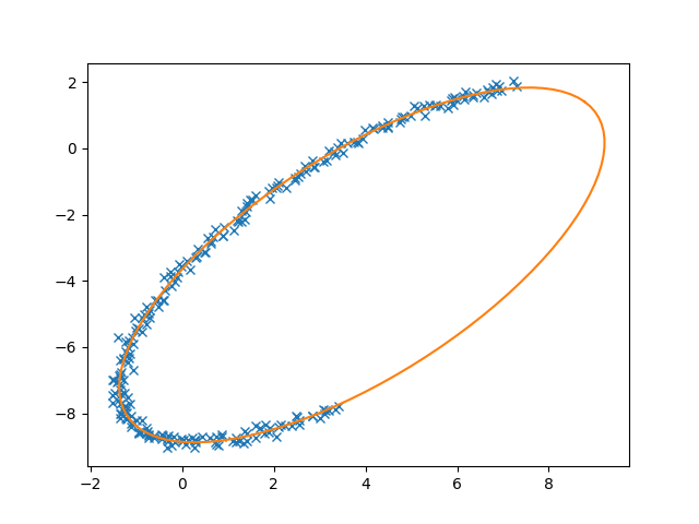
Note that the algorithm is inherently biased towards smaller ellipses because of its use of the algebraic distance as a metric for the goodness-of-fit rather than the geometric distance. As noted by both sources for the algorithm used in this post, this issue is discussed by Kanatani (1994) and is not easily overcome.

import numpy as np
import matplotlib.pyplot as plt


def fit_ellipse(x, y):
    """

    Fit the coefficients a,b,c,d,e,f, representing an ellipse described by
    the formula F(x,y) = ax^2 + bxy + cy^2 + dx + ey + f = 0 to the provided
    arrays of data points x=[x1, x2, ..., xn] and y=[y1, y2, ..., yn].

    Based on the algorithm of Halir and Flusser, "Numerically stable direct
    least squares fitting of ellipses'.


    """

    D1 = np.vstack([x**2, x*y, y**2]).T
    D2 = np.vstack([x, y, np.ones(len(x))]).T
    S1 = D1.T @ D1
    S2 = D1.T @ D2
    S3 = D2.T @ D2
    T = -np.linalg.inv(S3) @ S2.T
    M = S1 + S2 @ T
    C = np.array(((0, 0, 2), (0, -1, 0), (2, 0, 0)), dtype=float)
    M = np.linalg.inv(C) @ M
    eigval, eigvec = np.linalg.eig(M)
    con = 4 * eigvec[0]* eigvec[2] - eigvec[1]**2
    ak = eigvec[:, np.nonzero(con > 0)[0]]
    return np.concatenate((ak, T @ ak)).ravel()


def cart_to_pol(coeffs):
    """

    Convert the cartesian conic coefficients, (a, b, c, d, e, f), to the
    ellipse parameters, where F(x, y) = ax^2 + bxy + cy^2 + dx + ey + f = 0.
    The returned parameters are x0, y0, ap, bp, e, phi, where (x0, y0) is the
    ellipse centre; (ap, bp) are the semi-major and semi-minor axes,
    respectively; e is the eccentricity; and phi is the rotation of the semi-
    major axis from the x-axis.

    """

    # We use the formulas from https://mathworld.wolfram.com/Ellipse.html
    # which assumes a cartesian form ax^2 + 2bxy + cy^2 + 2dx + 2fy + g = 0.
    # Therefore, rename and scale b, d and f appropriately.
    a = coeffs[0]
    b = coeffs[1] / 2
    c = coeffs[2]
    d = coeffs[3] / 2
    f = coeffs[4] / 2
    g = coeffs[5]

    den = b**2 - a*c
    if den > 0:
        raise ValueError('coeffs do not represent an ellipse: b^2 - 4ac must'
                         ' be negative!')

    # The location of the ellipse centre.
    x0, y0 = (c*d - b*f) / den, (a*f - b*d) / den

    num = 2 * (a*f**2 + c*d**2 + g*b**2 - 2*b*d*f - a*c*g)
    fac = np.sqrt((a - c)**2 + 4*b**2)
    # The semi-major and semi-minor axis lengths (these are not sorted).
    ap = np.sqrt(num / den / (fac - a - c))
    bp = np.sqrt(num / den / (-fac - a - c))

    # Sort the semi-major and semi-minor axis lengths but keep track of
    # the original relative magnitudes of width and height.
    width_gt_height = True
    if ap < bp:
        width_gt_height = False
        ap, bp = bp, ap

    # The eccentricity.
    r = (bp/ap)**2
    if r > 1:
        r = 1/r
    e = np.sqrt(1 - r)

    # The angle of anticlockwise rotation of the major-axis from x-axis.
    if b == 0:
        phi = 0 if a < c else np.pi/2
    else:
        phi = np.arctan((2.*b) / (a - c)) / 2
        if a > c:
            phi += np.pi/2
    if not width_gt_height:
        # Ensure that phi is the angle to rotate to the semi-major axis.
        phi += np.pi/2
    phi = phi % np.pi

    return x0, y0, ap, bp, e, phi


def get_ellipse_pts(params, npts=100, tmin=0, tmax=2*np.pi):
    """
    Return npts points on the ellipse described by the params = x0, y0, ap,
    bp, e, phi for values of the parametric variable t between tmin and tmax.

    """

    x0, y0, ap, bp, e, phi = params
    # A grid of the parametric variable, t.
    t = np.linspace(tmin, tmax, npts)
    x = x0 + ap * np.cos(t) * np.cos(phi) - bp * np.sin(t) * np.sin(phi)
    y = y0 + ap * np.cos(t) * np.sin(phi) + bp * np.sin(t) * np.cos(phi)
    return x, y


if __name__ == '__main__':
    # Test the algorithm with an example elliptical arc.
    npts = 250
    tmin, tmax = np.pi/6, 4 * np.pi/3
    x0, y0 = 4, -3.5
    ap, bp = 7, 3
    phi = np.pi / 4
    # Get some points on the ellipse (no need to specify the eccentricity).
    x, y = get_ellipse_pts((x0, y0, ap, bp, None, phi), npts, tmin, tmax)
    noise = 0.1
    x += noise * np.random.normal(size=npts) 
    y += noise * np.random.normal(size=npts)

    coeffs = fit_ellipse(x, y)
    print('Exact parameters:')
    print('x0, y0, ap, bp, phi =', x0, y0, ap, bp, phi)
    print('Fitted parameters:')
    print('a, b, c, d, e, f =', coeffs)
    x0, y0, ap, bp, e, phi = cart_to_pol(coeffs)
    print('x0, y0, ap, bp, e, phi = ', x0, y0, ap, bp, e, phi)

    plt.plot(x, y, 'x')     # given points
    x, y = get_ellipse_pts((x0, y0, ap, bp, e, phi))
    plt.plot(x, y)
    plt.show()