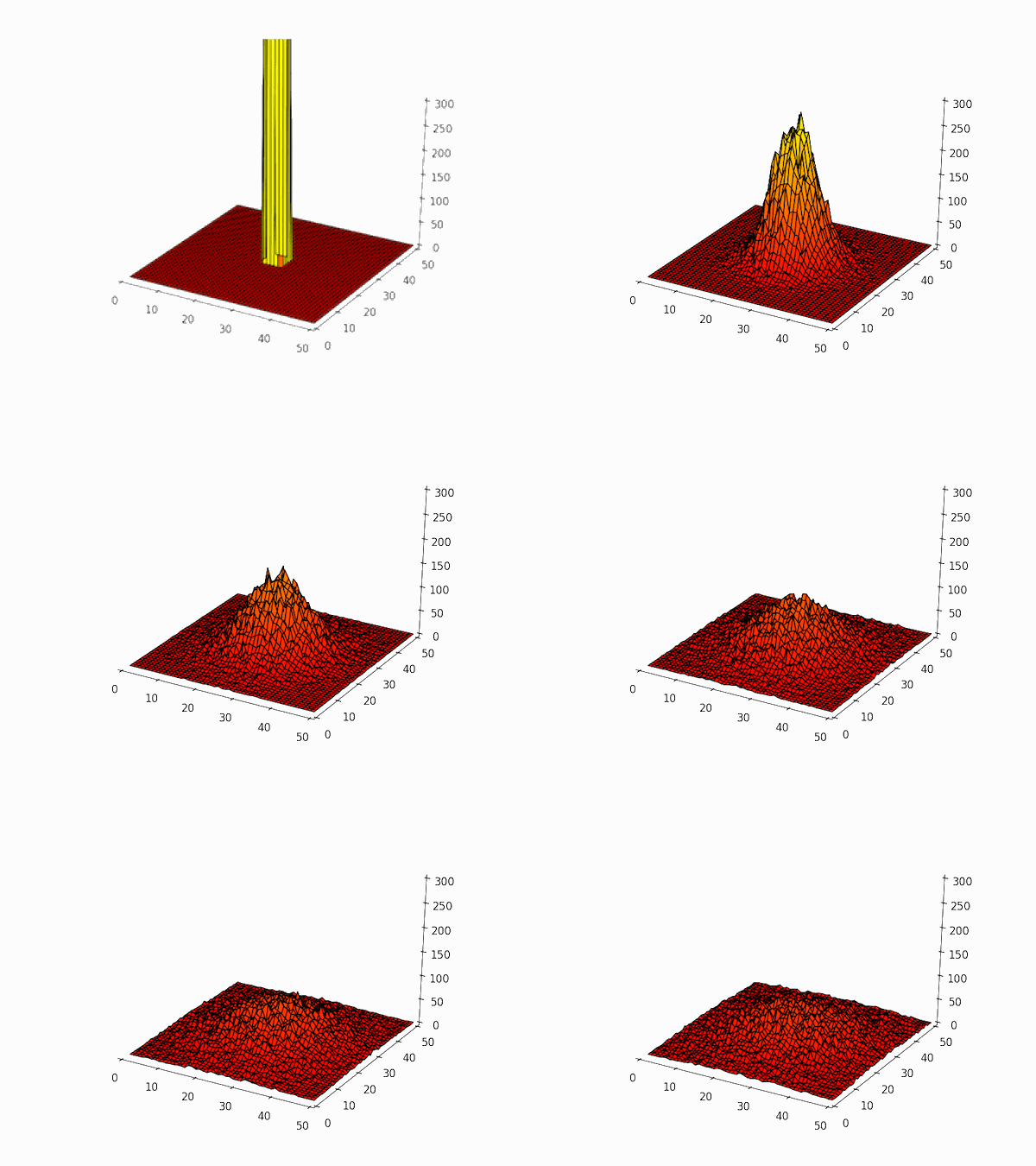
A very simple 2-D diffusion model

import numpy as np
import matplotlib.pyplot as plt
from mpl_toolkits.mplot3d import Axes3D
from matplotlib import  colors

# (Square) grid side length.
m = 50
# Maximum numbter of iterations.
nitmax = 200
# Number of particles in the simulation.
nparticles = 50000
# Output a frame (plot image) every nevery iterations.
nevery = 2
# Constant maximum value of z-axis value for plots.
zmax = 300

# Create the 3D figure object.
fig = plt.figure()
ax = fig.add_subplot(111, projection='3d')
# We'll need a meshgrid to plot the surface: this is X, Y.
x = y = np.linspace(1,m,m)
X, Y = np.meshgrid(x, y)

# vmin, vmax set the minimum and maximum values for the colormap. This is to
# be fixed for all plots, so define a suitable norm.
vmin, vmax = 0, zmax
norm = colors.Normalize(vmin=vmin, vmax=vmax)

# Initialize the location of all the particles to the centre of the grid.
locs = np.ones((nparticles, 2), dtype=int) * m//2

# Iterate for nitmax cycles.
for j in range(nitmax):
    # Update the particles' locations at random. Particles move at random to
    # an adjacent grid cell. We're going to be pretty relaxed about the ~11%
    # probability that a particle doesn't move at all (displacement of (0,0)).
    locs += np.random.randint(-1, 2, locs.shape)
    if not (j+1) % nevery:
        # Create an updated grid and plot it.
        grid = np.zeros((m, m))
        for i in range(nparticles):
            x, y = locs[i]
            # Add a particle to the grid if it is actually on the grid!
            if 0 <= x < m and 0 <= y < m:
                grid[x, y] += 1
        print(j+1,'/',nitmax)
        # Now clear the Axes of any previous plot and make a new surface plot.
        ax.clear()
        ax.plot_surface(X, Y, grid, rstride=1, cstride=1, cmap=plt.cm.autumn,
                        linewidth=1, vmin=vmin, vmax=vmax, norm=norm)
        ax.set_zlim(0, zmax)
        # Save to 'diff-000.png', 'diff-001.png', ...
        plt.savefig('diff-{:03d}.png'.format(j//nevery))