The tumbling of Hyperion · scipython.com

P8.2.7The tumbling of Hyperion

Hyperion is an irregularly-shaped moon of Saturn notable for its chaotic rotation. Its motion may be modelled as follows.

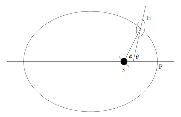
The orbit of Hyperion (H) about Saturn (S) is an ellipse with semi-major axis, $$a$$ , and eccentricity, $$e$$ . Let its point of closest approach (periapsis) be P. Its distance from the planet, SH, as a function of its true anomaly (orbital angle, $\phi$ , measured from the line SP) is therefore

r = \frac{a(1-e^2)}{1+e\cos\phi}.

Define the angle $\theta$ to be that between the axis of the smallest principal moment of inertia (loosely, the longest axis of the moon) and SP, and the quantity $\Omega$ to be a scaled rate of change of $\theta$ with $\phi$ (i.e. the rate at which Hyperion spins as it orbits Saturn) as follows:

\Omega = \frac{a^2}{r^2}\frac{\mathrm{d}\theta}{\mathrm{d}\phi}.

Now, it can be shown that

\frac{\mathrm{d}\Omega}{\mathrm{d}\phi} = - \frac{B-A}{C}\frac{3}{2(1-e^2)}\frac{a}{r}\sin [2(\theta-\phi)],

where $$A$$ , $$B$$ and $$C$$ are the principal moments of inertia.

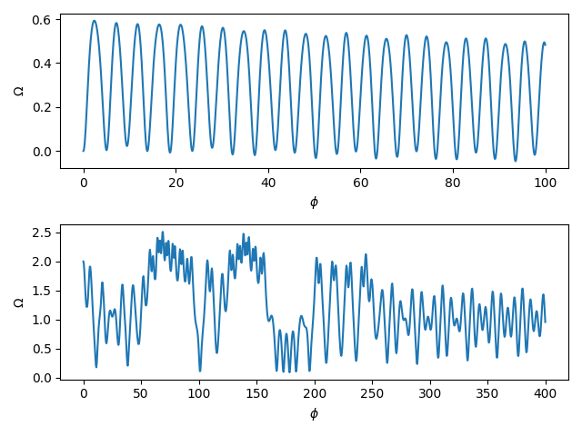
Use scipy.integrate.odeint to find and plot the spin rate, $\Omega$ , as a function of $\phi$ for the initial conditions (a) $\theta = \Omega = 0$ at $\phi = 0$ , and (b) $\theta = 0$ , $\Omega = 2$ at $\phi=0$ . Take $$e=0.1$$ and $$(B-A)/C = 0.265$$ .

Show solution

The following code demonstrates the chaotic tumbling behaviour of Hyperion at under some conditions.

hyperiontumbling

import numpy as np
from matplotlib import pyplot as plt
from scipy.integrate import solve_ivp

# The orbital eccentricity, e, and (B-A)/C for Hyperion
e, BmAoC = 0.1, 0.265

# Anonymous function for calculating a/r as a function of true anomaly, phi
a_over_r = lambda phi: (1 + e * np.cos(phi)) / (1 - e**2)


def deriv(phi, z):
    """
    Given z = Omega, theta, calculate and return the derivatives,
    dOmega/dphi and dtheta/dphi.

    """

    Omega, theta = z
    aor = a_over_r(phi)
    theta_d = aor**-2 * Omega
    Omega_d = -BmAoC * 3 / 2 / (1 - e**2) * aor * np.sin(2 * (theta - phi))
    return Omega_d, theta_d


fig, axes = plt.subplots(nrows=2, ncols=1)

# Different pairs of initial conditions.
z0 = [(0, 0), (2, 0)]
phimax = [100, 400]

for i in range(2):
    soln = solve_ivp(deriv, (0, phimax[i]), z0[i], dense_output=True)
    phi = np.linspace(0, phimax[i], 1000)
    Omega, theta = soln.sol(phi)
    axes[i].plot(phi, Omega)
    axes[i].set_xlabel(r"$\phi$")
    axes[i].set_ylabel(r"$\Omega$")

fig.tight_layout()
plt.show()

The motion of Hyperion under two sets of initial conditions: $\theta = \Omega = 0$ (top) and $\theta = 0$ , $\Omega = 2$ (bottom).