Modelling a radioactive decay chain

P8.2.8Modelling a radioactive decay chain

The radioactive decay chain of $\mathrm{^{212}Pb}$ to the stable isotope $\mathrm{^{208}Pb}$ may be considered as the following sequence of steps with the given rate constants, $$k_i$$ :

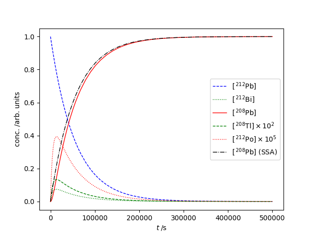
\begin{align*} \mathrm{^{212}Pb} & \rightarrow \mathrm{^{212}Bi} + \beta^- & \quad k_1 &= 1.816 \times 10^{-5}\;\mathrm{s^{-1}},\\ \mathrm{^{212}Bi} & \rightarrow \mathrm{^{208}Tl} + \alpha & \quad k_2 &= 6.931 \times 10^{-5}\;\mathrm{s^{-1}},\\ \mathrm{^{212}Bi} & \rightarrow \mathrm{^{212}Po} + \beta^- & \quad k_3 &= 1.232 \times 10^{-4}\;\mathrm{s^{-1}},\\ \mathrm{^{208}Tl} & \rightarrow \mathrm{^{208}Pb} + \beta^- & \quad k_4 &= 3.851 \times 10^{-3}\;\mathrm{s^{-1}},\\ \mathrm{^{212}Po} & \rightarrow \mathrm{^{208}Pb} + \alpha & \quad k_5 &= 2.310 \;\mathrm{s^{-1}}. \end{align*}

By considering the following first-order differential equations giving the rates of change for each species, plot their concentrations as a function of time.

\begin{align*} \frac{\mathrm{d[^{212}Pb]}}{\mathrm{d}t} &= -k_1 \mathrm{[^{212}Pb]}\\ \frac{\mathrm{d[^{212}Bi]}}{\mathrm{d}t} &= k_1 \mathrm{[^{212}Pb]} - k_2 \mathrm{[^{212}Bi]} - k_3 \mathrm{[^{212}Bi]}\\ \frac{\mathrm{d[^{208}Tl]}}{\mathrm{d}t} &= k_2 \mathrm{[^{212}Bi]} - k_4 \mathrm{[^{208}Tl]}\\ \frac{\mathrm{d[^{212}Po]}}{\mathrm{d}t} &= k_3 \mathrm{[^{212}Bi]} - k_5 \mathrm{[^{212}Po]}\\ \frac{\mathrm{d[^{208}Pb]}}{\mathrm{d}t} &= k_4 \mathrm{[^{208}Tl]} + k_5 \mathrm{[^{212}Po]} \end{align*}

If all the intermediate species, J, are treated in "steady state" (i.e. $\mathrm{d[J]}/\mathrm{d}t = 0$ , the approximate expression for the $\mathrm{^{208}Pb}$ concentration as a function of time is

[\mathrm{^{208}Pb}] = [\mathrm{^{212}Pb}]_0 \left(1-e^{-k_1t}\right).

Compare the "exact" result obtained by numerical integration of above the differential equations with this approximate answer.

Show solution

Although we could invoke the steady-state approximation (at least for $\mathrm{[^{208}Tl]}$ and $\mathrm{[^{212}Po]}$ ) to reduce the number of differential equations, the code below integrates them all.

radioactivedecaychain

import numpy as np
from scipy.integrate import solve_ivp
import matplotlib.pyplot as plt

species = ["212Pb", "212Bi", "208Tl", "212Po", "208Pb"]

# The decay processes and their indexes in the list of rate coefficients, k
# 0: 212Pb -> 212Bi + beta-
# 1: 212Bi -> 208Tl + alpha
# 2: 212Bi -> 212Po + beta-
# 3: 208Tl -> 208Pb + beta-
# 4: 212Po -> 208Pb + alpha
k = [1.816e-05, 6.931e-05, 1.232e-4, 3.851e-3, 2.310]


def deriv(t, X):
    """Return dX/dt for each of the species."""
    return (
        -k[0] * X[0],  # 212Pb
        k[0] * X[0] - k[1] * X[1] - k[2] * X[1],  # 212Bi
        k[1] * X[1] - k[3] * X[2],  # 208Tl
        k[2] * X[1] - k[4] * X[3],  # 212Po
        k[3] * X[2] + k[4] * X[3],  # 208Pb
    )


# Initial conditions: only 212Pb present
X0 = [1, 0, 0, 0, 0]
# Integrate the differential equations for tf secs
tf = 5.0e5
soln = solve_ivp(deriv, (0, tf), X0, method="LSODA")
t = soln.t
X = soln.y
plt.plot(t, X[0], label=r"$[\,\mathrm{^{212}Pb}]$", c="b", ls="--", lw=1)
plt.plot(t, X[1], label=r"$[\,\mathrm{^{212}Bi}]$", c="g", ls=":", lw=1)
plt.plot(t, X[4], label=r"$[\,\mathrm{^{208}Pb}]$", c="r", lw=1)
plt.plot(
    t,
    X[2] * 1.0e2,
    label=r"$[\,\mathrm{^{208}Tl}] \times 10^{2}$",
    c="g",
    ls="--",
    lw=1,
)
plt.plot(
    t,
    X[3] * 1.0e5,
    label=r"$[\,\mathrm{^{212}Po}] \times 10^{5}$",
    c="r",
    ls=":",
    lw=1,
)

Css = 1 - np.exp(-k[0] * t)  # all intermediates in steady-state
plt.plot(t, Css, c="k", ls="-.", label=r"$[\,\mathrm{^{208}Pb}]$ (SSA)", lw=1)

plt.legend()
plt.xlabel(r"$t\;/\mathrm{s}$")
plt.ylabel(r"conc. /arb. units")
plt.show()

Concentrations of various isotopes in the decay chain originating with (212Pb).