Modelling the evolution of a match flame

P8.2.9Modelling the evolution of a match flame

A simple model of the evolution of a match flame considers the flame radius, $$y$$ , to change in time as

\frac{\mathrm{d}y}{\mathrm{d}t} = \alpha y^2 - \beta y^3,

where $\alpha$ and $\beta$ are some constants relating to the transport of oxygen through the surface of the flame and the rate of its consumption inside it. The flame is initally small, $y(0) \ll \alpha/\beta$ , but at some point rapidly grows until it reaches a steady state of constant radius (assuming an unlimited supply of fuel).

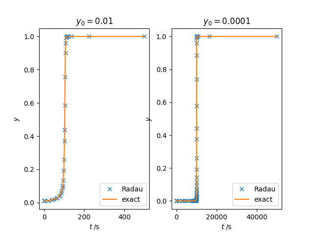
Taking $\alpha=\beta=1$ , solve this ODE numerically using scipy.integrate.solve_ivp using a suitable integration method over a time interval $$(0, 5/y(0))$$ for (a) $$y(0) = 0.01$$ , (b) $$y(0) = 0.0001$$ . How many time steps must be taken in each case?

The exact solution may be written as

y(t) = \frac{\alpha}{\beta\left[1+W\left(a\mathrm{e}^{a-\alpha^2t/\beta}\right)\right]},

where $a=\alpha/(\beta y(0))$ and $$W(x)$$ is the Lambert $$W$$ function, implemented in SciPy as scipy.special.lambertw. Compare the accuracy of the various numerical solutions with this expression.

Show solution

Here is one solution. The 'Radau' solver (an implicit Runge-Kutta method) is suitable, and requires 262 function evaluations for $$y(0) = 0.01$$ and 546 at $$y(0) = 0.0001$$ .

matchflame

import numpy as np
from scipy.integrate import solve_ivp
from scipy.special import lambertw
import matplotlib.pyplot as plt

method = "Radau"


def solve_flame_eqn(alpha, beta, y0):
    def dydt(t, y):
        ydot = y**2 * (alpha - beta * y)
        return ydot

    t0, tf = 0, 5 / y0
    # Integrate the differential equation.
    sol = solve_ivp(dydt, (t0, tf), [y0], method=method)
    t, y = sol.t, sol.y[0]

    print(f"alpha/beta = {alpha / beta}, y(0) = {y0}: nfev = {sol.nfev}")
    return t, y


def make_plot(ax, t, y):
    a = alpha / beta / y0 - 1
    yW = alpha / beta / (1 + lambertw(a * np.exp(a - alpha**2 * t / beta)))
    ax.plot(t, y, "x", label=method)
    ax.plot(t, yW, label="exact")
    ax.set_xlabel(r"$t \;/\mathrm{s}$")
    ax.set_ylabel(r"$y$")
    ax.legend()


fig, axes = plt.subplots(nrows=1, ncols=2)

alpha, beta = 1, 1

y0 = 0.01
t, y = solve_flame_eqn(alpha, beta, y0)
make_plot(axes[0], t, y)
axes[0].set_title(r"$y_0 = 0.01$")

y0 = 1.0e-4
t, y = solve_flame_eqn(alpha, beta, y0)
make_plot(axes[1], t, y)
axes[1].set_title(r"$y_0 = 0.0001$")

plt.show()