The Chapman cycle · scipython.com

P8.2.6The Chapman cycle

A simple mechanism for the formation of ozone in the stratosphere consists of the following four reactions (known as the Chapman cycle):

\begin{align*} \mathrm{O_2} + h\nu & \rightarrow 2\mathrm{O} & k_1 = 3 \times 10^{-12}\;\mathrm{s^{-1}}\\ \mathrm{O_2} + \mathrm{O} + \mathrm{M} & \rightarrow \mathrm{O_3} + \mathrm{M} & k_2 = 1.2\times 10^{-33}\;\mathrm{cm^6\,molec^{-2}\,s^{-1}}\\ \mathrm{O_3} + h\nu' & \rightarrow \mathrm{O} + \mathrm{O_2} & k_3 = 5.5 \times 10^{-4}\;\mathrm{s^{-1}}\\ \mathrm{O} + \mathrm{O_3} & \rightarrow 2\mathrm{O_2} & k_4 = 6.9\times 10^{-16}\;\mathrm{cm^3\,molec^{-1}\,s^{-1}} \end{align*}

where M is a non-reacting third-body taken to be at the total air molecule concentration for the altitude being considered. The above reactions lead to the following rate equations for $\mathrm{[O]}$ , $\mathrm{[O_3]}$ and $\mathrm{[O_2]}$ :

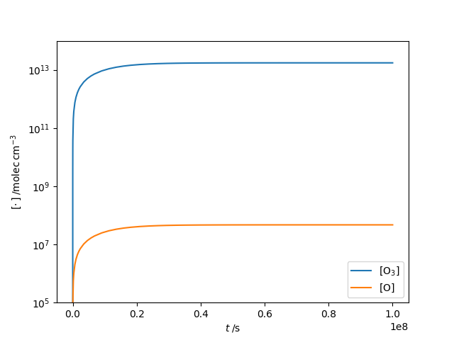
\begin{align*} \frac{\mathrm{d[O_2]}}{\mathrm{d}t} &= -k_1\mathrm{[O_2]} - k_2\mathrm{[O_2]}\mathrm{[O]}\mathrm{[M]} + k_3\mathrm{[O_3]} + 2k_4\mathrm{[O]}\mathrm{[O_3]}\\ \frac{\mathrm{d[O]}}{\mathrm{d}t} &= 2k_1\mathrm{[O_2]} - k_2\mathrm{[O_2]}\mathrm{[O]}\mathrm{[M]} + k_3\mathrm{[O_3]} - k_4\mathrm{[O]}\mathrm{[O_3]}\\ \frac{\mathrm{d[O_3]}}{\mathrm{d}t} &= k_2\mathrm{[O_2]}\mathrm{[O]}\mathrm{[M]} - k_3\mathrm{[O_3]} - k_4\mathrm{[O]}\mathrm{[O_3]} \end{align*}

The above rate constants apply at an altitude of 25 km, where $\mathrm{[M]} = 9\times 10^{17}\;\mathrm{molec\,cm^{-3}}$ . Write a program to determine the concentrations of $\mathrm{O_3}$ and $\mathrm{O}$ as a function of time at this altitude (you should find the $\mathrm{[O_2]}$ remains pretty much constant). Start with initial conditions $\mathrm{[O_2]_0} = 0.21\mathrm{[M]}$ , $\mathrm{[O]_0} = \mathrm{[O_3]_0} = 0$ and integrate for $10^8\;\mathrm{s}$ (starting from scratch it takes about 3 years to build an ozone layer with this mechanism). Compare the equilibrium concentrations with the approximate analytical result obtained using the steady-state approximation:

\mathrm{[O_3]} = \sqrt{\frac{k_1k_2}{k_3k_4}}\mathrm{[O_2]}\mathrm{[M]}^\frac{1}{2}, \quad \frac{\mathrm{[O]}}{\mathrm{[O_3]}} = \frac{k_3}{k_2\mathrm{[O_2]}\mathrm{[M]}}.

Show solution

The code below uses scipy.integrate.solve_ivp to solve the three coupled differential equations describing the concentrations of $\mathrm{O_2}$ , $\mathrm{O}$ and $\mathrm{O_3}$ with time.

chapmancycle

import numpy as np
from scipy.integrate import solve_ivp
import matplotlib.pyplot as plt

# Reaction rate constants.
k1 = 3.0e-12  #    O2 + hv -> 2O      (s-1)
k2 = 1.2e-33  # O2 + O + M -> O3 + M  (cm6.molec-2.s-1)
k3 = 5.5e-4  #   O3 + hv' -> O + O2  (s-1)
k4 = 6.9e-16  #     O + O3 -> 2O2     (cm3.molec-1.s-1)


def deriv(t, c, M):
    """Return the d[X]/dt for each species."""
    O2, O, O3 = c
    dO2dt = -k1 * O2 - k2 * M * O * O2 + k3 * O3 + 2 * k4 * O * O3
    dOdt = 2 * k1 * O2 - k2 * M * O * O2 + k3 * O3 - k4 * O * O3
    dO3dt = k2 * M * O * O2 - k3 * O3 - k4 * O * O3
    return dO2dt, dOdt, dO3dt


# Total molecule concentration, M, and O2 concentration, cO2.
M = 9.0e17
cO2 = 0.21 * M
# Initial conditions for [O2], [O], [O3]
c0 = [cO2, 0, 0]
# Integrate the differential equations over a suitable time grid (s).
ti, tf = 0, 1.0e8
# NB We need a solver that is robust to stiff ODEs.
soln = solve_ivp(deriv, (ti, tf), c0, args=(M,), method="LSODA")
t, c = soln.t, soln.y

# Steady-state approximation solution for comparison.
cO3ss = np.sqrt(k1 * k2 / k3 / k4 * M) * cO2
cOss = k3 * cO3ss / k2 / cO2 / M

cO, cO3 = c[1, -1], c[2, -1]
print("Numerical values:")
print(f"[O] = {cO:g} molec/cm3, [O3] = {cO3:g} molec/cm3")
print("Steady-state values:")
print(f"[O]ss = {cOss:g} molec/cm3, [O3]ss = {cO3ss:g} molec/cm3")

# Plot the evolution of [O3] and [O] with time
plt.plot(t, c[2], label=r"$\mathrm{[O_3]}$")
plt.plot(t, c[1], label=r"$\mathrm{[O]}$")
plt.yscale("log")
plt.ylim(1.0e5, 1.0e14)
plt.xlabel(r"$t\;/\mathrm{s}$")
plt.ylabel(r"$[\cdot\,]\;/\mathrm{molec\,cm^{-3}}$")
plt.legend()
plt.show()

The output shows that the steady-state approximation works well at this altitude:

Numerical values:
[O] = 4.70561e+07 molec/cm3, [O3] = 1.74604e+13 molec/cm3
Steady-state values:
[O]ss = 4.7055e+07 molec/cm3, [O3]ss = 1.74634e+13 molec/cm3