The general pendulum · scipython.com

P8.2.5The general pendulum

The equation governing the motion of a pendulum consisting of a mass $$m$$ at the end of a light, rigid rod of length $$l$$ may be written

\frac{\mathrm{d}^2\theta}{\mathrm{d}t^2} = -\frac{g}{l}\sin\theta,

where $\theta$ is the angle the pendulum makes with the vertical.

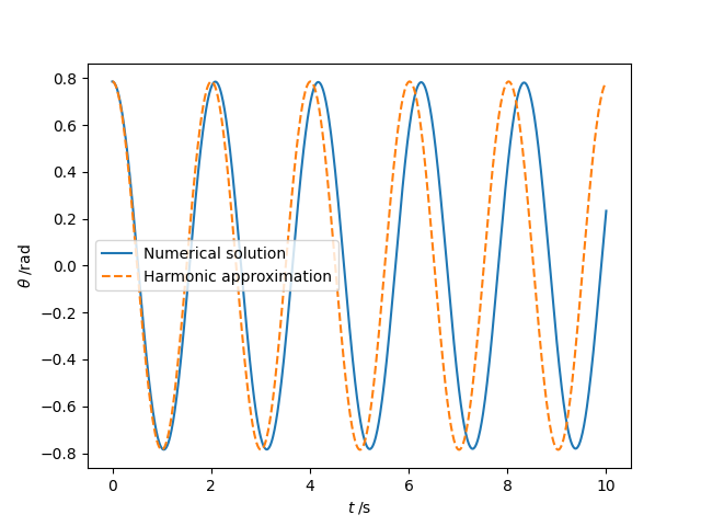
Taking $l=1\;\mathrm{m}$ and $g=9.81\;\mathrm{m\,s^{-2}}$ , determine the subsequent motion of the pendulum if it is started at rest with an initial angle $\theta_0 = 30^\circ$ . Compare the motion with the harmonic approximation reached by assuming $\theta$ is small which has the analytical solution $\theta = \theta_0\cos(\omega t)$ with $\omega = \sqrt{g/l}$ .

Show solution

The provided second-order differential equation can, in fact, be wrangled into a single first-order differential equation but we choose here to reduce it to two such equations in variables $\theta$ and $\dot{\theta}$ :

\begin{align*} \frac{\mathrm{d}\dot{\theta}}{\mathrm{d}t} &= -\frac{g}{l}\sin\theta,\\ \frac{\mathrm{d}\theta}{\mathrm{d}t} &= \dot{\theta}. \end{align*}

generalpendulum

import numpy as np
from scipy.integrate import solve_ivp
import matplotlib.pyplot as plt

# Acceleration due to gravity (m.s-2), pendulum length (m).
g, l = 9.81, 1
omega = np.sqrt(g / l)
omega2 = omega**2

# Initial conditions.
theta0, theta_dot0 = np.radians(45), 0
y0 = (theta0, theta_dot0)


def deriv(t, y, omega2):
    """Return the derivatives dtheta/dt, d2theta/dt2."""
    theta, theta_dot = y
    return theta_dot, -omega2 * np.sin(theta)


# Integrate the differential equation from ti to tf secs.
ti, tf = 0, 10
soln = solve_ivp(deriv, (ti, tf), y0, args=(omega2,), dense_output=True)

# A suitable grid of time points.
t = np.linspace(ti, tf, 1000)
theta = soln.sol(t)[0]

# Small angle approximation - harmonic motion.
theta_harmonic = theta0 * np.cos(omega * t)

plt.plot(t, theta, label="Numerical solution")
plt.plot(t, theta_harmonic, ls="--", label="Harmonic approximation")
plt.xlabel(r"$t\;/\mathrm{s}$")
plt.ylabel(r"$\theta\;/\mathrm{rad}$")
plt.legend()
plt.show()

Comparison of the numerical solution of the pendulum equation with its harmonic approximation.