The Brusselator · scipython.com

P8.2.4The Brusselator

The Brusselator is a theoretical model for an autocatalytic reaction. It assumes the following reaction sequence, in which species A and B are taken to be in excess with constant concentration and species D and E are removed as they are produced. The concentrations of species X and Y can show oscillatory behaviour under certain conditions.

\begin{align*} \mathrm{A} & \rightarrow \mathrm{X} & \quad k_1\\ 2\mathrm{X} + \mathrm{Y} & \rightarrow 3\mathrm{X} & \quad k_2\\ \mathrm{B} + \mathrm{X} & \rightarrow \mathrm{Y} + \mathrm{D} & \quad k_3\\ \mathrm{X} & \rightarrow \mathrm{E} & \quad k_4 \end{align*}

It is convenient to introduce the scaled quantities

\begin{align*} x = [\mathrm{X}]\sqrt{\frac{k_2}{k_4}}, & \quad y = [\mathrm{Y}]\sqrt{\frac{k_2}{k_4}},\\ a = [\mathrm{A}]\frac{k_1}{k_4}\sqrt{\frac{k_2}{k_4}}, & \quad b = [\mathrm{B}]\frac{k_3}{k_4}, \end{align*}

and to scale the time by the factor $$k_4$$ , which gives rise to the dimensionless equations

\begin{align*} \frac{\mathrm{d}x}{\mathrm{d}t} &= a - (1+b)x + x^2y,\\ \frac{\mathrm{d}y}{\mathrm{d}t} &= bx - x^2y. \end{align*}

Starting with $$x(0) = y(0) = 1$$ , show how these equations predict $$x$$ and $$y$$ to vary for (a) $$a = 1, b = 1.8$$ and (b) $$a = 1, b = 2.02$$ by plotting in each case (i) $$x,y$$ as functions of (dimensionless) time and (ii) $$y$$ as a function of $$x$$ .

Show solution

We can integrate the two coupled ordinary differential equations with scipy.integrate.odeint() and plot the results in two different ways for the two sets of parameter values, $$(a,b)$$ .

brusselator

import numpy as np
from scipy.integrate import solve_ivp
from matplotlib import pyplot as plt

fig, axes = plt.subplots(nrows=2, ncols=2)


def deriv(t, X, a, b):
    """Return the derivatives dx/dt and dy/dt."""
    x, y = X
    dxdt = a - (1 + b) * x + x**2 * y
    dydt = b * x - x**2 * y
    return dxdt, dydt


x0, y0 = 1, 1


def plot_brusselator(a, b, row):
    """
    Integrate the Brusselator equations for parameters a,b and plot."""

    ti, tf = 0, 100
    soln = solve_ivp(
        deriv, (ti, tf), (x0, y0), dense_output=True, args=(a, b)
    )

    t = np.linspace(ti, tf, 1000)
    X = soln.sol(t)
    ax_left = axes[row, 0]
    ax_left.plot(t, X[0], lw=1)
    ax_left.plot(t, X[1], lw=1)
    ax_left.legend((r"$x$", r"$y$"), loc="upper right")
    ax_left.set_xlabel(r"$t$")
    ax_right = axes[row, 1]
    ax_right.plot(X[0], X[1], c="b", lw=1)
    ax_right.set_xlabel(r"$x$")
    ax_right.set_ylabel(r"$y$")


# Integrate and plot the Brusselator for each of the parameter pairs (1, 1.8)
# and (1, 2.02); the results from each calculation is plotted on a single row
# of the figure identified by row=0 or row=1
plot_brusselator(1, 1.8, 0)
plot_brusselator(1, 2.02, 1)

fig.tight_layout()
plt.show()

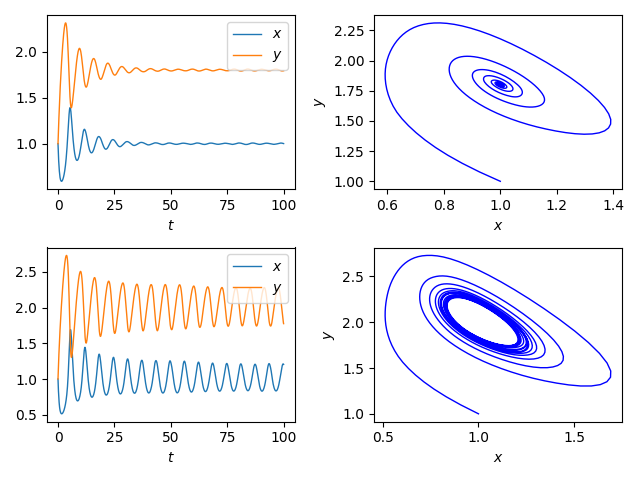
This system displays an Andronov-Hopf bifurcation at $b_\star=a^2 + 1$ : for $$b$$ less this value (top two plots) there is a stable focus: the concentrations of X and Y converge on stable equilibrium values; for $b > b_\star$ the system enters a limit cycle (bottom two plots).