The two-dimensional advection equation

P7.5.3The two-dimensional advection equation

The two-dimensional advection equation may be written

\frac{\partial U}{\partial t} = -v_x\frac{\partial U}{\partial x} - v_y\frac{\partial U}{\partial y},

where $\boldsymbol{v} = (v_x, v_y)$ is the vector velocity field giving the velocity components $$v_x$$ and $$v_y$$ , which may vary as a function of position, $$(x, y)$$ . In a similar way to the approach taken in Example E7.23, this equation may be discretized and solved numerically. With forward-differences in time and central-differences in space, we have

u_{i,j}^{(n+1)} = u_{i,j}^{(n)} - \Delta t \left[ v_{x;i,j}\frac{u_{i+1,j}^{(n)} - u_{i-1,j}^{(n)}}{2\Delta x} + v_{y;i,j}\frac{u_{i,j+1}^{(n)} - u_{i,j-1}^{(n)}}{2\Delta y}\right].

Implement this approximate numerical solution on the domain $0\le x < 10, 0\le y< 10$ discretized with $\Delta x = \Delta y = 0.1$ with the initial condition

u_0(x,y) = \exp\left( - \frac{(x-c_x)^2 + (y-c_y)^2}{\alpha^2}\right),

where $$(c_x, c_y) = (5, 5)$$ and $\alpha = 2$ . Take the velocity field to be a circulation at constant speed $$0.05$$ about an origin at $$(7,5)$$ .

Show solution

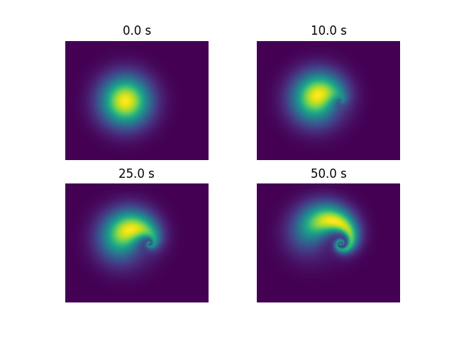
The following program produces some pleasing swirls upon advection of the initial function.

advection2d

import numpy as np
import matplotlib.pyplot as plt

randint = np.random.randint

# Domain size
w = h = 10.0
w = 12
# Intervals in x-, y- directions
dx = dy = 0.1
nx, ny = int(w / dx), int(h / dy)
# Time interval
dt = 0.01

# The discretized function on the domain. Note that rows (first index)
# correspond to the y-axis and columns (second index) to the x-index
u0 = np.zeros((ny, nx))
u = np.zeros((ny, nx))
x, y = np.meshgrid(np.arange(0, nx * dx, dx), np.arange(0, ny * dy, dy))
# Initial state: a two-dimensional Gaussian function
cx, cy, alpha = 5, 5, 2
u0 = np.exp(-((x - cx) ** 2 + (y - cy) ** 2) / alpha**2)

# A two-dimensional vector field discretized on our domain
cx, cy, v0 = 7, 5, 0.05
# (rx, ry) is the vector from the vortex centre to the point (x,y)
rx, ry = x - cx, y - cy
r = np.hypot(rx, ry)
# v = v0 * normalized unit vector perpendicular to r is (-ry, rx), indexed
# by row, column as (vy, vx)
v = v0 * np.dstack((rx, -ry)) / r[..., np.newaxis]
v[np.isnan(v)] = 0


def do_timestep(u0, u):
    # forward-difference in time, central-difference in space numerical
    # solution to the 2D advection equation
    u[1:-1, 1:-1] = (
        u0[1:-1, 1:-1]
        - dt
        * (
            v[1:-1, 1:-1, 1]
            * (u0[1:-1, 2:] - u0[1:-1, :-2])
            / 2
            / dx  # vx.du/dx
            + v[1:-1, 1:-1, 0] * (u0[2:, 1:-1] - u0[:-2, 1:-1]) / 2 / dy
        )
    )  # vy.du/dy

    u0 = u.copy()
    return u0, u


# Number of timesteps:
nsteps = 5001
# Output 4 figures at these timesteps
mfig = [0, 1000, 2500, 5000]
fignum = 0
fig = plt.figure()
for m in range(nsteps):
    u0, u = do_timestep(u0, u)
    if m in mfig:
        fignum += 1
        print(m, fignum)
        ax = fig.add_subplot(220 + fignum)
        im = ax.imshow(u.copy())
        ax.set_axis_off()
        ax.set_title(f"{m * dt:.1f} s")
plt.show()