P7.4.4Atmospheric carbon dioxide concentrations
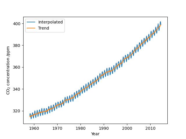
The United States The National Oceanic and Atmospheric Administration (NOAA) releases a freely-available data set of atmospheric carbon dioxide concentrations since 1958. Using this data, plot the "interpolated'' and "trend'' \(\mathrm{CO_2}\) concentration against time on the same graph.
Show solution
The following program plots the specified atmospheric \(\mathrm{CO_2}\) concentration data over time on a graph.
atmosphericco2
import numpy as np
import matplotlib.pyplot as plt

dt = np.dtype([("date", "f8"), ("co2_ppm", "f8"), ("co2_ppm_trend", "f8")])
data = np.loadtxt("co2_mm_mlo.txt", usecols=(2, 4, 5), dtype=dt)

fig, ax = plt.subplots()
ax.plot(data["date"], data["co2_ppm"], label="Interpolated")
ax.plot(data["date"], data["co2_ppm_trend"], label="Trend")
ax.set_xlabel("Year")
ax.set_ylabel(r"$\mathrm{CO_2}$ concentration /ppm")
ax.legend(loc=0)  # Legend in the "best" position
plt.show()