The Brachistochrone problem

The Brachistochrone problem asks the question "what is the shape of the curve down which a bead sliding from rest and accelerated by gravity will slip, without friction, from one fixed point, $$P_1$$ to another $$P_2$$ in the least time?"

Its solution is well-known and given in various forms in many places on the internet, but is given in outline at the bottom of this post.

Paths between $$P_1 = (0,0)$$ and $$P_2 = (1, 0.65)$$ :

enter image description here

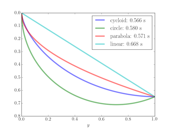
Note that the path giving the shortest time (the cycloid) is not the shortest distance between the points and may have a minimum (i.e. the bead slides down and then up before reaching $$P_2$$ , as shown by the following example for $$P_2 = (1, 0.3)$$ .

enter image description here

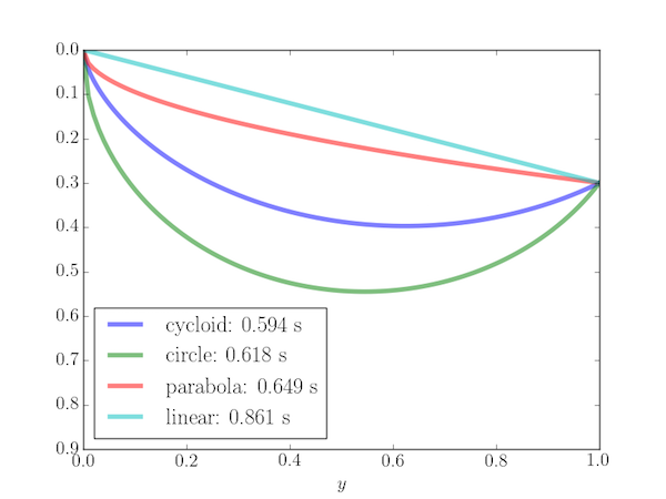
The following Python program plots the Brachistochrone curve (an arc of a cycloid) and calculates the time of travel. It is also compared with three other paths: (i) a straight line, (ii) a circular path with a vertical tangent at $$P_1$$ and (iii) a parabola with vertical tangent at $$P_1$$ .

import numpy as np
from scipy.optimize import newton
from scipy.integrate import quad
import matplotlib.pyplot as plt

# Acceleration due to gravity (m.s-2); final position of bead (m).
g = 9.81
x2, y2 = 1, 0.65

def cycloid(x2, y2, N=100):
    """Return the path of Brachistochrone curve from (0,0) to (x2, y2).

    The Brachistochrone curve is the path down which a bead will fall without
    friction between two points in the least time (an arc of a cycloid).
    It is returned as an array of N values of (x,y) between (0,0) and (x2,y2).

    """

    # First find theta2 from (x2, y2) numerically (by Newton-Rapheson).
    def f(theta):
        return y2/x2 - (1-np.cos(theta))/(theta-np.sin(theta))
    theta2 = newton(f, np.pi/2)

    # The radius of the circle generating the cycloid.
    R = y2 / (1 - np.cos(theta2))

    theta = np.linspace(0, theta2, N)
    x = R * (theta - np.sin(theta))
    y = R * (1 - np.cos(theta))

    # The time of travel
    T = theta2 * np.sqrt(R / g)
    print('T(cycloid) = {:.3f}'.format(T))
    return x, y, T

def linear(x2, y2, N=100):
    """Return the path of a straight line from (0,0) to (x2, y2)."""

    m = y2 / x2
    x = np.linspace(0, x2, N)
    y = m*x

    # The time of travel
    T = np.sqrt(2*(1+m**2)/g/m * x2)
    print('T(linear) = {:.3f}'.format(T))
    return x, y, T

def func(x, f, fp):
    """The integrand of the time integral to be minimized for a path f(x)."""

    return np.sqrt((1+fp(x)**2) / (2 * g * f(x)))

def circle(x2, y2, N=100):
    """Return the path of a circular arc between (0,0) to (x2, y2).

    The circle used is the one with a vertical tangent at (0,0).

    """

    # Circle radius
    r = (x2**2 + y2**2)/2/x2

    def f(x):
        return np.sqrt(2*r*x - x**2)
    def fp(x):
        return (r-x)/f(x)

    x = np.linspace(0, x2, N)
    y = f(x)

    # Calcualte the time of travel by numerical integration.
    T = quad(func, 0, x2, args=(f, fp))[0]
    print('T(circle) = {:.3f}'.format(T))
    return x, y, T

def parabola(x2, y2, N=100):
    """Return the path of a parabolic arc between (0,0) to (x2, y2).

    The parabola used is the one with a vertical tangent at (0,0).

    """

    c = (y2/x2)**2

    def f(x):
        return np.sqrt(c*x)
    def fp(x):
        return c/2/f(x)

    x = np.linspace(0, x2, N)
    y = f(x)

    # Calcualte the time of travel by numerical integration.
    T = quad(func, 0, x2, args=(f, fp))[0]
    print('T(parabola) = {:.3f}'.format(T))
    return x, y, T

# Plot a figure comparing the four paths.
fig, ax = plt.subplots()

for curve in ('cycloid', 'circle', 'parabola', 'linear'):
    x, y, T = globals()[curve](x2, y2)
    ax.plot(x, y, lw=4, alpha=0.5, label='{}: {:.3f} s'.format(curve, T))
ax.legend()

ax.set_xlabel('$x$')
ax.set_xlabel('$y$')
ax.set_xlim(0, 1)
ax.set_ylim(0.8, 0)
plt.savefig('brachistochrone.png')
plt.show()

Appendix A: Solution the the Brachistochrone problem

We choose $$P_1 = (0,0)$$ and set $$P_2 = (x_2, y_2)$$ , with the $$y-$$ axis pointing in the same direction as the acceleration due to gravity, $\boldsymbol{g}$ . Then we seek to minimize

T = \int_{P_1}^{P_2}\frac{\mathrm{d}s}{v},

where the arc length element along the curve we seek is $\mathrm{d}s = \sqrt{\mathrm{d}x^2 + \mathrm{d}y^2}$ and the speed along the curve, $$v$$ satisfies $\frac{1}{2}mv^2 = mgy$ by conservation of energy. Then the functional to be minimized is

T = \int_{P_1}^{P_2}\sqrt{\frac{1+y'^2}{2gy}}\,\mathrm{d}x,

where $y' = \mathrm{d}y/\mathrm{d}x$ . The function to be varied in this minimization,

F(x,y,y') = \sqrt{\frac{1+y'^2}{2gy}}

does not explicitly depend on $$x$$ so the Beltrami identity applies:

F - y'\frac{\partial F}{\partial y'} = C = \mathrm{constant}.

Now,

\frac{\partial F}{\partial y'} = \frac{y'}{\sqrt{2gy}\sqrt{1+y'^2}}

and substitution into the Beltrami identity gives

y(1+y'^2) = \frac{1}{2gC^2} = 2R.

This differential equation has a parametric solution in the form of a cycloid:

\begin{align*} x(\theta) &= R(\theta - \sin\theta),\\ y(\theta) &= R(1 - \cos\theta). \end{align*}

The parameter $\theta$ varies from $$0$$ at $$P_1 = (0,0)$$ to $\theta_2$ at $$P_2 = (x_2, y_2)$$ which may be found numerically as the solution to

\frac{y_2}{x_2} = \frac{1-\cos\theta_2}{\theta_2 - \sin\theta_2}

Substitution back into the second parametric equation then gives

R = \frac{y_2}{1-\cos\theta_2}.

Appendix B: Paths and times for other curves

Straight line

The straight line between $$P_1 = (0,0)$$ and $$P_2 = (x_2,y_2)$$ has the equation $$y = mx$$ with $$m=y_2/x_2$$ . The time taken is

T = \int_{P_1}^{P_2}\sqrt{\frac{1+y'^2}{2gy}}\,\mathrm{d}x = \int_0^{x_2} \sqrt{\frac{1+m^2}{2gmx}}\,\mathrm{d}x = \sqrt{\frac{(1+m^2)x_2}{gm}}.

Circular arc

The circle through $$P_1 = (0,0)$$ and $$P_2 = (x_2,y_2)$$ with vertical tangent at $$P_1$$ has the formula $$y^2 = r^2 - (x-r)^2$$ with radius

r = \frac{x_2^2 + y_2^2}{2x_2}.

The integral giving $$T$$ may be evaluated numerically using $y = \sqrt{2xr-x^2}$ and $$y' = (r-x)/y$$ .

Parabolic arc

The parabola through $$P_1 = (0,0)$$ and $$P_2 = (x_2,y_2)$$ with vertical tangent at $$P_1$$ has the formula $y = \sqrt{cx}$ with $$c = (y_2/x_2)^2$$ . The integral giving $$T$$ may be evaluated numerically using this and $$y' = c/(2y)$$ .