Reaching Orbit
Posted on 22 October 2018
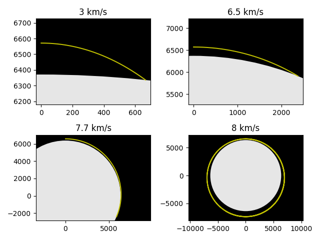
The following code illustrates the effect of the initial velocity on the dynamics of an object released in a gravitational field. A very simple numerical integration of the equation of motion gives the trajectory, which is plotted below for four different initial speeds for a rocket released at 200 km altitude parallel to the Earth's surface. At this altitude the speed needed for a circular orbit is about 7.8 km/s. You can read more about this kind of simulation at the Wikipedia page for Newton's cannonball.
The velocity and position are calculated from the acceleration at each time step of the simulation, which is taken to be due to the force of gravity only (a ballistic trajectory):
$$ \mathbf{a} = -\frac{GM}{r^3}\mathbf{r}, $$ where $M$ is the mass of the planet.
Note that atmospheric drag and the Earth's own rotation are neglected.
import numpy as np
import matplotlib.pyplot as plt
from matplotlib.patches import Circle

from scipy.constants import G
# Convert Newtonian constant of gravitation from m3.kg-1.s-2 to km3.kg-1.s-2
G /= 1.e9

# Planet radius, km
R = 6371
# Planet mass, kg
M = 5.9722e24

fac = G * M
def calc_a(r):
    """Calculate the acceleration of the rocket due to gravity at position r."""
    r3 = np.hypot(*r)**3
    return -fac * r / r3

def get_trajectory(h, launch_speed, launch_angle):
    """Do the (very simple) numerical integration of the equation of motion.

    The satellite is released at altitude h (km) with speed launch_speed (km/s)
    at an angle launch_angle (degrees) from the normal to the planet's surface.

    """

    v0 = launch_speed
    theta = np.radians(launch_angle)

    N = 100000
    tgrid, dt = np.linspace(0, 15000, N, retstep=True)
    tr = np.empty((N,2))
    v = np.empty((N,2))
    # Initial rocket position, velocity and acceleration
    tr[0] = 0, R + h
    v[0] = v0 * np.sin(theta), v0 * np.cos(theta)
    a = calc_a(tr[0])

    for i, t in enumerate(tgrid[1:]):
        # Calculate the rocket's next position based on its instantaneous velocity.
        r = tr[i] + v[i]*dt
        if np.hypot(*r) < R:
            # Our rocket crashed.
            break
        # Update the rocket's position, velocity and acceleration.
        tr[i+1] = r
        v[i+1] = v[i] + a*dt
        a = calc_a(tr[i+1])

    return tr[:i+1]

# Rocket initial speed (km.s-1), angle from local vertical (deg)
launch_speed, launch_angle = 2.92, 90
# Rocket launch altitute (km)
h = 200
tr = get_trajectory(h, launch_speed, launch_angle)

def plot_trajectory(ax, tr):
    """Plot the trajectory tr on Axes ax."""
    earth_circle = Circle((0,0), R, facecolor=(0.9,0.9,0.9))
    ax.set_facecolor('k')
    ax.add_patch(earth_circle)
    ax.plot(*tr.T, c='y')
    # Make sure our planet looks circular!
    ax.axis('equal')

    # Set Axes limits to trajectory coordinate range, with some padding.
    xmin, xmax = min(tr.T[0]), max(tr.T[0])
    ymin, ymax = min(tr.T[1]), max(tr.T[1])
    dx, dy = xmax - xmin, ymax - ymin
    PAD = 0.05
    ax.set_xlim(xmin - PAD*dx, xmax + PAD*dx)
    ax.set_ylim(ymin - PAD*dy, ymax + PAD*dy)

fig, axes = plt.subplots(nrows=2, ncols=2)
for i, launch_speed in enumerate([3, 6.5, 7.7, 8]):
    tr = get_trajectory(h, launch_speed, launch_angle)
    ax = axes[i//2,i%2]
    plot_trajectory(ax, tr)
    ax.set_title('{} km/s'.format(launch_speed))
plt.tight_layout()

plt.savefig('orbit.png')
plt.show()