The scipy.optimize.curve_fit routine can be used to fit two-dimensional data, but the fitted data (the ydata argument) must be repacked as a one-dimensional array first. The independent variable (the xdata argument) must then be an array of shape (2,M) where M is the total number of data points.

For a two-dimensional array of data, Z, calculated on a mesh grid (X, Y), this can be achieved efficiently using the ravel method:

xdata = np.vstack((X.ravel(), Y.ravel()))
ydata = Z.ravel()

The following code demonstrates this approach for some synthetic data set created as a sum of four Gaussian functions with some noise added:

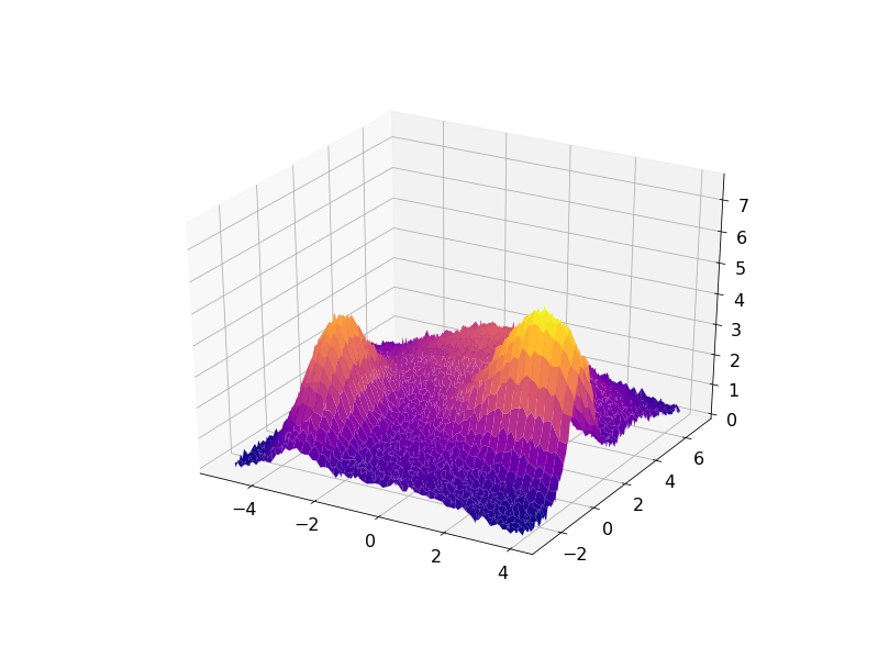
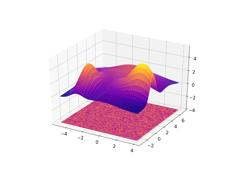
The result can be visualized in 3D with the residuals plotted on a plane under the fitted data:

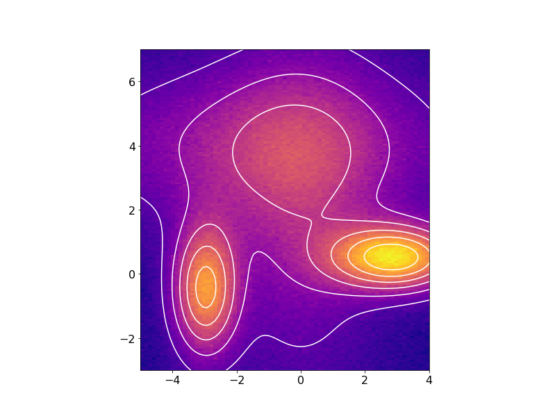
or in 2D with the fitted data contours superimposed on the noisy data:

import numpy as np
from scipy.optimize import curve_fit
import matplotlib.pyplot as plt
from mpl_toolkits.mplot3d import Axes3D

# The two-dimensional domain of the fit.
xmin, xmax, nx = -5, 4, 75
ymin, ymax, ny = -3, 7, 150
x, y = np.linspace(xmin, xmax, nx), np.linspace(ymin, ymax, ny)
X, Y = np.meshgrid(x, y)

# Our function to fit is going to be a sum of two-dimensional Gaussians
def gaussian(x, y, x0, y0, xalpha, yalpha, A):
    return A * np.exp( -((x-x0)/xalpha)**2 -((y-y0)/yalpha)**2)

# A list of the Gaussian parameters: x0, y0, xalpha, yalpha, A
gprms = [(0, 2, 2.5, 5.4, 1.5),
         (-1, 4, 6, 2.5, 1.8),
         (-3, -0.5, 1, 2, 4),
         (3, 0.5, 2, 1, 5)
        ]

# Standard deviation of normally-distributed noise to add in generating
# our test function to fit.
noise_sigma = 0.1

# The function to be fit is Z.
Z = np.zeros(X.shape)
for p in gprms:
    Z += gaussian(X, Y, *p)
Z += noise_sigma * np.random.randn(*Z.shape)

# Plot the 3D figure of the fitted function and the residuals.
fig = plt.figure()
ax = fig.gca(projection='3d')
ax.plot_surface(X, Y, Z, cmap='plasma')
ax.set_zlim(0,np.max(Z)+2)
plt.show()

# This is the callable that is passed to curve_fit. M is a (2,N) array
# where N is the total number of data points in Z, which will be ravelled
# to one dimension.
def _gaussian(M, *args):
    x, y = M
    arr = np.zeros(x.shape)
    for i in range(len(args)//5):
       arr += gaussian(x, y, *args[i*5:i*5+5])
    return arr

# Initial guesses to the fit parameters.
guess_prms = [(0, 0, 1, 1, 2),
              (-1.5, 5, 5, 1, 3),
              (-4, -1, 1.5, 1.5, 6),
              (4, 1, 1.5, 1.5, 6.5)
             ]
# Flatten the initial guess parameter list.
p0 = [p for prms in guess_prms for p in prms]

# We need to ravel the meshgrids of X, Y points to a pair of 1-D arrays.
xdata = np.vstack((X.ravel(), Y.ravel()))
# Do the fit, using our custom _gaussian function which understands our
# flattened (ravelled) ordering of the data points.
popt, pcov = curve_fit(_gaussian, xdata, Z.ravel(), p0)
fit = np.zeros(Z.shape)
for i in range(len(popt)//5):
    fit += gaussian(X, Y, *popt[i*5:i*5+5])
print('Fitted parameters:')
print(popt)

rms = np.sqrt(np.mean((Z - fit)**2))
print('RMS residual =', rms)

# Plot the 3D figure of the fitted function and the residuals.
fig = plt.figure()
ax = fig.gca(projection='3d')
ax.plot_surface(X, Y, fit, cmap='plasma')
cset = ax.contourf(X, Y, Z-fit, zdir='z', offset=-4, cmap='plasma')
ax.set_zlim(-4,np.max(fit))
plt.show()

# Plot the test data as a 2D image and the fit as overlaid contours.
fig = plt.figure()
ax = fig.add_subplot(111)
ax.imshow(Z, origin='bottom', cmap='plasma',
          extent=(x.min(), x.max(), y.min(), y.max()))
ax.contour(X, Y, fit, colors='w')
plt.show()