Posted by: christian on 24 Aug 2015
Having built a database of UK house "paid price" data as described in a previous blog post, we can do some analysis. From within PostgreSQL, one can do straighforward things like get a property's price history. For example:
house_prices=# SELECT date_of_transfer, price, paon, postcode FROM pp
               WHERE paon='37' AND postcode='ME10 3AY'
               ORDER BY date_of_transfer;
 date_of_transfer | price  | paon | postcode
------------------+--------+------+----------
 1998-01-23       |  65750 | 37   | ME10 3AY
 2001-08-22       |  89995 | 37   | ME10 3AY
 2003-08-22       | 137000 | 37   | ME10 3AY
 2007-06-01       | 169995 | 37   | ME10 3AY
(4 rows)
But more sophisticated analysis of average trends is harder work in pure SQL and can be done from Python using the psycopg2 module. The following code allows search constraints to be passed on the command line using the argparse module, part of the Python 3 standard library. It returns the median values of properties meeting these constraints, either over each year (the default) or each month (by specifying the -m option.)
# get_medians.py
import sys
import psycopg2
import numpy as np
import argparse

# Argument parser: specify constraints and medians timeframe on command line
parser = argparse.ArgumentParser(description='Return median house prices'
                                         ' over time given some constraints.')
parser.add_argument('--postcode', type=str,
                    help='Postcode or initial fragment of a postcode')
parser.add_argument('--paon', type=str,
                    help='Primary addressable object name, e.g. house number')
parser.add_argument('--town', type=str, dest='town_city',
                    help='Town or city name')
parser.add_argument('--city', type=str, dest='town_city',
                    help='Town or city name')
timeframe = parser.add_mutually_exclusive_group()
timeframe.add_argument('-y', action='store_true', default=True,
                    help='Calculate median within each year')
timeframe.add_argument('-m', action='store_true', default=False,
                    help='Calculate median within each month')

constraints = parser.parse_args()
sql_constraints = ['']
if constraints.paon:
    sql_constraints.append("paon='{0:s}'".format(constraints.paon))
if constraints.town_city:
    sql_constraints.append("town_city='{0:s}'".format(
                       constraints.town_city.upper()))
if constraints.postcode:
    sql_constraints.append("postcode LIKE '{:s}%'".format(constraints.postcode))
sql_constraints = ' AND '.join(sql_constraints)

def increment_month(year, month):
    """Increment the date given by year, month by one month."""
    month += 1
    if month == 13:
        year, month = year + 1, 1
    return year, month

def increment_year(year, month):
    """Increment the date given by year, month by one year."""
    year += 1
    return year, month

# Select the required time interval increment function (+1 month or +1 year)
increment_time_interval = increment_year
if constraints.m:
    increment_time_interval = increment_month

conn = psycopg2.connect(database='house_prices', user='<USERNAME>',
                        password='<PASSWORD>')
cursor = conn.cursor()

end_year, end_month = 2015, 1
year1, month1 = 1995, 1
while (year1, month1) != (end_year, end_month):
    year2, month2 = increment_time_interval(year1, month1)
    date_start = '{0:4d}-{1:02d}-01'.format(year1, month1)
    date_end = '{0:4d}-{1:02d}-01'.format(year2, month2)
    query = "SELECT price from pp WHERE date_of_transfer >= '{0:s}' AND"\
            " date_of_transfer < '{1:s}'{2:s}".format(
                    date_start, date_end, sql_constraints)

    cursor.execute(query)
    prices = np.array(cursor.fetchall())
    median_price = np.median(prices)
    print('{0:s} {1:d} {2:.2f}'.format(date_start, len(prices), median_price))

    year1, month1 = year2, month2
Note that this script is intended for personal use only and makes no attempt to protect against SQL injection and the like (i.e. don't run it on your public-facing server!) The columns returned are the date, number of transactions and median price paid.
For example, the median house price in Cambridge each year is returned with:
$ python get_medians.py --city=Cambridge
1995-01-01 3464 71500.00
1996-01-01 4328 75000.00
1997-01-01 5058 84000.00
1998-01-01 4375 93000.00
1999-01-01 4908 104000.00
2000-01-01 4813 123500.00
2001-01-01 4910 140000.00
2002-01-01 4832 165000.00
2003-01-01 4821 180000.00
2004-01-01 4597 195000.00
2005-01-01 4594 210000.00
2006-01-01 5524 220000.00
2007-01-01 5109 247000.00
2008-01-01 3065 235000.00
2009-01-01 3384 220000.00
2010-01-01 3717 245000.00
2011-01-01 3761 249995.00
2012-01-01 3509 250000.00
2013-01-01 4261 279950.00
2014-01-01 4576 299995.00
To plot these data, redirect the output for several cities to text files called median-<city>.txt and use the following program, plot_medians.py:
# plot_medians.py
import sys
import numpy as np
import pandas as pd
import matplotlib.pyplot as plt
from matplotlib.ticker import FuncFormatter

import matplotlib

cities = sys.argv[1:]

dateparse = lambda s: pd.datetime.strptime(s, '%Y-%m-%d')
fig = plt.figure(facecolor='w')
ax = fig.add_subplot(111, axisbg='w')

for city in cities:
    filename = 'median-{}.txt'.format(city.lower())
    df = pd.read_table(filename,
                       names=('month', 'n', 'median_price'), sep=' ')
    df.month = df.month.apply(dateparse)

    ax.plot(df['month'], df['median_price'], lw=2, marker='o', markersize=8,
            markeredgecolor='w', alpha=0.7, label=city.title())

ax.tick_params(length=5, width=2, direction='out', color='#cccccc')
ax.yaxis.grid(color='#cccccc', linestyle='-', lw=2)

ax.xaxis.tick_bottom()
ax.yaxis.tick_left()
ymajorFormatter = FuncFormatter(lambda val,pos: '£{:3d}k'.format(int(val/1000)))
ax.yaxis.set_major_formatter(ymajorFormatter)
ax.set_ylim(0,455000)
xlims = ax.get_xlim()
xlim_pad = 100      # days
ax.set_xlim(xlims[0]-xlim_pad, xlims[1]+xlim_pad)

for pos in ax.spines:
    ax.spines[pos].set_visible(False)

ax.legend(loc='upper left')
ax.set_axisbelow(True)

ax.set_title('Median House prices since 1995')
#plt.show()
For example,
python plot_medians.py Oxford Newport York Cambridge London
produces the depressing (if you want to live in London and don't currently own a house) plot:

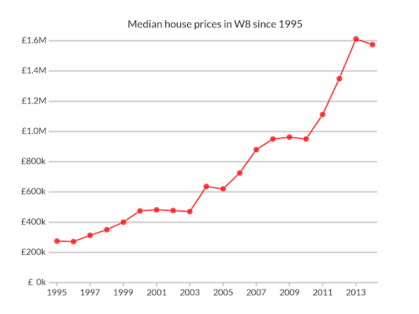
Searching on partial postcodes is also supported:
$ python get_medians.py --postcode "W8"
1995-01-01 490 275000.00
1996-01-01 677 271500.00
...
2013-01-01 348 1612500.00
2014-01-01 355 1575000.00
People who bought houses in Kensington 20 years ago seem to have made a lot of money.

Comments
Comments are pre-moderated. Please be patient and your comment will appear soon.
There are currently no comments
New Comment