Modelling an antenna array

An antenna array can be used to direct radio waves in a particular direction by adjusting their number, geometrical arrangement, and relative amplitudes and phases (see e.g. S. J. Orfanidis, Electromagnetic Waves and Antennas, Rutgers University, 2016.)

Consider an array of $$n$$ isotropic antennas at positions, $\boldsymbol{d}_i$ , evenly spaced by $$d$$ along the $$x$$ -axis from the origin:

\begin{align*} \boldsymbol{d}_0 = 0, \boldsymbol{d}_1 = d\boldsymbol{\hat{x}}, \ldots,\boldsymbol{d}_{n-1} = (n-1)d\boldsymbol{\hat{x}}. \end{align*}

If a single antenna produces a radiation vector, $\boldsymbol{F}(\boldsymbol{k})$ , where $\boldsymbol{k} = k\boldsymbol{\hat{r}} = (2\pi/\lambda)\boldsymbol{\hat{r}}$ , the total radiation vector due to all $$n$$ antennas is

\begin{align*} \boldsymbol{F}_\mathrm{tot}(\boldsymbol{k}) = \sum_{j=0}^{n-1}w_j\mathrm{e}^{ji\boldsymbol{k}\cdot\boldsymbol{d}_j}\boldsymbol{F}(\boldsymbol{k}) = A(\boldsymbol{k})F(\boldsymbol{k}), \end{align*}

where $$w_j$$ is the feed coefficient of the $$j$$ th antenna, representing its amplitude and phase, and $A(\boldsymbol{k})$ is known as the array factor. We can choose $$w_0 = 1$$ to specify the feed coefficients relative to the antenna at the origin. If we further choose to look only at the azimuthal ( $\phi$ ) contribution to the radiation in the $$xy$$ plane, setting the polar angle $\theta=\pi/2$ , we have:

A(\phi) = \sum_{j=0}^{n-1}w_j\mathrm{e}^{jikd\cos\phi}.

The relative radiation power pattern ("gain") is the square of this quantity. For two identical antennas,

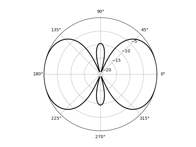
g(\phi) = |A(\phi)|^2 = |w_0 + w_1\mathrm{e}^{ikd\cos\phi}|^2.

In the code below, the related quantity, the directive gain, $10\log_{10}(g/g_\mathrm{max})$ , is plotted below as a function of $\phi$ for the two-antenna case on a polar plot for $d=\lambda$ and $$w_0 =1, w_1 = -i$$ .

antennaarray1

import numpy as np
import matplotlib.pyplot as plt


def gain(d, w):
    """Return the power as a function of azimuthal angle, phi."""
    phi = np.linspace(0, 2 * np.pi, 1000)
    psi = 2 * np.pi * d / lam * np.cos(phi)
    A = w[0] + w[1] * np.exp(1j * psi)
    g = np.abs(A) ** 2
    return phi, g


def get_directive_gain(g, minDdBi=-20):
    """Return the "directive gain" of the antenna array producing gain g."""
    DdBi = 10 * np.log10(g / np.max(g))
    return np.clip(DdBi, minDdBi, None)


# Wavelength, antenna spacing, feed coefficients.
lam = 1
d = lam
w = np.array([1, -1j])
# Calculate gain and directive gain; plot on a polar chart.
phi, g = gain(d, w)
DdBi = get_directive_gain(g)

plt.polar(phi, DdBi, c="k", lw=2)
ax = plt.gca()
ax.set_rticks([-20, -15, -10, -5])
ax.set_rlabel_position(45)
plt.show()

Notes:

To better show the interesting region of the plot, where the power is highest, we "clip" the values less than minDdBi to that value.
To customize the plot we need the Axes object in the current plot context; this is returned by plt.gca() ("get current axes").
set_rticks sets the position of the radial tick marks.
set_rlabel_position defines the angular position of the radial ticks.

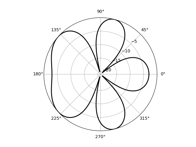
The directive gain of a two-antenna array with d = lambda, w0 = 1;w1 = -i — The directive gain of a two-antenna array with $d = \lambda, w_0 = 1; w_1 = -i$ .

NumPy's broadcasting methods provide a natural way to extend this code to an arbitrary number of antennas; in the following example the figure method add_subplot is called with the argument projection='polar' and returns a corresponding Axes object, ax.

antennaarray2

import numpy as np
import matplotlib.pyplot as plt


def gain(d, w):
    """Return the power as a function of azimuthal angle, phi."""
    phi = np.linspace(0, 2 * np.pi, 1000)
    psi = 2 * np.pi * d / lam * np.cos(phi)
    j = np.arange(len(w))
    A = np.sum(w[j] * np.exp(j * 1j * psi[:, None]), axis=1)
    g = np.abs(A) ** 2
    return phi, g


def get_directive_gain(g, minDdBi=-20):
    """Return the "directive gain" of the antenna array producing gain g."""
    DdBi = 10 * np.log10(g / np.max(g))
    return np.clip(DdBi, minDdBi, None)


# Wavelength, antenna spacing, feed coefficients.
lam = 1
d = lam / 2
w = np.array([1, -1, 1])
# Calculate gain and directive gain; plot on a polar chart.
phi, g = gain(d, w)
DdBi = get_directive_gain(g)

fig = plt.figure()
ax = fig.add_subplot(projection="polar")
ax.plot(phi, DdBi, c="k", lw=2)
ax.set_rticks([-20, -15, -10, -5])
ax.set_rlabel_position(45)
plt.show()

The sum to calculate $$A$$ is over the terms in the array factor expression: adding an axis to thepsi array calculates this sum for each of the angular positions, $\phi$ .

Note that with the projection already defined, we need ax.plot here, not ax.polar to plot the data.

The directive gain of a many-antenna array with d = lambda/2, w0 = 1;w1 = -1;w2 = 1 — The directive gain of a many-antenna array with $d = \lambda/2, w_0 = 1;w_1 = -1;w_2 = 1$ .

E7.12Modelling an antenna array