Visualizing linear transformations

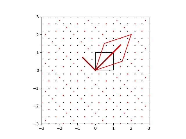
A linear transformation in two dimensions can be visualized through its effect on the unit square defined by the two orthonormal basis vectors, $\boldsymbol{\hat{\imath}}$ and $\boldsymbol{\hat{\jmath}}$ . In general, it can be represented by a $2\times 2$ matrix, $\mathbf{T}$ , which acts on a vector $\boldsymbol{v}$ to map it from a vector space spanned by one basis onto a different vector space spanned by another basis: $\boldsymbol{v'} = \mathbf{T}\boldsymbol{v}$ . Eigenvectors under such a transformation may be scaled but do not change orientation, as illustrated by the following code for the transformation matrix:

\begin{align*} \mathbf{T} = \left( \begin{array}{rr} \frac{3}{2} & \frac{1}{2}\\[1ex] \frac{1}{2} & \frac{3}{2} \end{array} \right). \end{align*}

The effect of the transformation on a set of points in the Cartesian plane is also visualized in the output plot below.

Visualizing a linear transformation in the Cartesian plane.

visualizinglineartransform

import numpy as np
import matplotlib.pyplot as plt

# Set up a Cartesian grid of points.
XMIN, XMAX, YMIN, YMAX = -3, 3, -3, 3
N = 16
xgrid = np.linspace(XMIN, XMAX, N)
ygrid = np.linspace(YMIN, YMAX, N)
grid = np.array(np.meshgrid(xgrid, ygrid)).reshape(2, N**2)

# Our untransformed unit basis vectors, i and j:
basis = np.array([[1, 0], [0, 1]])


def plot_quadrilateral(basis, color="k"):
    """Plot the quadrilateral defined by the two basis vectors."""
    ix, iy = basis[0]
    jx, jy = basis[1]
    plt.plot([0, ix, ix + jx, jx, 0], [0, iy, iy + jy, jy, 0], color)


def plot_vector(v, color="k", lw=1):
    """Plot vector v as a line with a specified color and linewidth."""
    plt.plot([0, v[0]], [0, v[1]], c=color, lw=lw)


def plot_points(grid, color="k"):
    """Plot the grid points in a specified color."""
    plt.scatter(*grid, c=color, s=2)


def apply_transformation(basis, T):
    """Return the transformed basis after applying transformation T."""
    return (T @ basis.T).T


# The untransformed grid and unit square.
plot_points(grid)
plot_quadrilateral(basis)

# Apply the transformation matrix, S, to the scene.
S = np.array(((1.5, 0.5), (0.5, 1.5)))
tbasis = apply_transformation(basis, S)
plot_quadrilateral(tbasis, "r")
tgrid = S @ grid
plot_points(tgrid, "r")

# Find the eigenvalues and eigenvectors of S...
vals, vecs = np.linalg.eig(S)
print(vals, vecs)
if all(np.isreal(vals)):
    # ... if they're all real, indicate them on the diagram.
    v1, v2 = vals
    e1, e2 = vecs.T
    plot_vector(v1 * e1, "r", 3)
    plot_vector(v2 * e2, "r", 3)
    plot_vector(e1, "k")
    plot_vector(e2, "k")

# Ensure the plot has 1:1 aspect (i.e. squares look square) and set the limits.
plt.axis("square")
plt.xlim(XMIN, XMAX)
plt.ylim(YMIN, YMAX)

plt.show()

Note that we need to reshape the meshgrid of $N\,\times\,N$ points into an array of $2\,\times\,N^2$ coordinates with:

grid = np.array(np.meshgrid(xgrid, ygrid)).reshape(2, N**2)

so that grid can be transformed in a single line of code by the vectorized operation, S @ grid.

E6.16Visualizing linear transformations