Fitting the Beer-Lambert law with NumPy

The Beer-Lambert law relates the concentration, $$c$$ , of a substance in a solution sample to the intensity of light transmitted through the sample, $I_\mathrm{t}$ across a given path length, $$l$$ , at a given wavelength, $\lambda$ :

I_\mathrm{t} = I_0 e^{-\alpha c l},

where $$I_0$$ is the incident light intensity and $\alpha$ is the absorption coefficient at $\lambda$ .

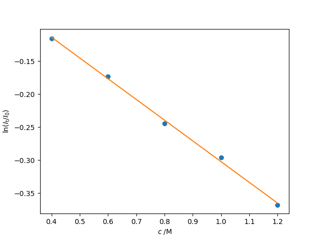
Given a series of measurements of the fraction of light transmitted, $I_\mathrm{t}/I_0$ , $\alpha$ may be determined through a least-squares fit to the straight line:

y = \ln\frac{I_\mathrm{t}}{I_0} = -\alpha c l.

Although this line passes through the origin ( $$y=0$$ for $$c=0$$ ), we will fit the more general linear relationship:

\[y = mc + k\]

where $m = -\alpha l$ , and verify that $$k$$ is close to zero.

Given a sample with path length $l = 0.8\;\mathrm{cm}$ , the following data were measured for $I_\mathrm{t}/I_0$ at five different concentrations:

$c\;/\mathrm{M}$	$I_\mathrm{t}/I_0$
0.4	0.886
0.6	0.833
0.8	0.784
1.0	0.738
1.2	0.694

The matrix form of the least squares equation to be solved is

\begin{align*} \left(\begin{array}{ll} c_1 & 1\\ c_2 & 1\\ c_3 & 1\\ c_4 & 1\\ c_5 & 1\\ \end{array}\right) \left(\begin{array}{l} m \\ k \end{array}\right) = \left(\begin{array}{ll} T_1\\ T_2\\ T_3\\ T_4\\ T_5\\ \end{array}\right) \end{align*}

where $T = \ln(I_\mathrm{t}/I_0)$ . The code below determines $$m$$ and hence $\alpha$ using np.linalg.lstsq:

beerlambertfit

import numpy as np
import matplotlib.pyplot as plt

# Path length, cm
path = 0.8
# The data: concentrations (M) and It/I0
c = np.array([0.4, 0.6, 0.8, 1.0, 1.2])
It_over_I0 = np.array([0.891, 0.841, 0.783, 0.744, 0.692])

n = len(c)
A = np.vstack((c, np.ones(n))).T
T = np.log(It_over_I0)

x, resid, _, _ = np.linalg.lstsq(A, T, rcond=None)
m, k = x
alpha = -m / path
print(f"alpha = {alpha:.3f} M-1.cm-1")
print("k", k)
print("rms residual = ", np.sqrt(resid[0]))

plt.plot(c, T, "o")
plt.plot(c, m * c + k)
plt.xlabel("$c\;/\mathrm{M}$")
plt.ylabel("$\ln(I_\mathrm{t}/I_0)$")
plt.show()

Here, _ is the dummy variable name conventionally given to an object we do not need to store or use.

The output produces a best fit value of $\alpha=0.393\;\mathrm{M^{-1}\,cm^{-1}}$ and a value of $$k$$ compatible with experimental error:

alpha = 0.393 M-1.cm-1
k 0.0118109033334
rms residual =  0.0096843591966

Least-squares fitting to the Beer-Lambert Law.

E6.17Fitting the Beer-Lambert law with NumPy