Mesh analysis of a electrical network

The currents flowing in the closed regions labelled $$I_1$$ , $$I_2$$ and $$I_3$$ of the circuit given below may be analysed by mesh analysis.

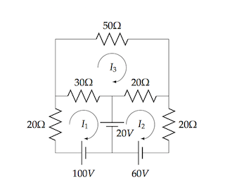
For each closed loop, we can apply Kirchoff's Voltage Law, $\sum_k V_k = 0$ , in conjunction with Ohm's Law, $$V = IR$$ , to give three simultaneous equations:

\begin{align*} 50I_1 - 30I_3 &= 80,\\ 40I_2 - 20I_3 &= 80,\\ -30I_1 - 20I_2 + 100I_3 &= 0. \end{align*}

These can be expressed in matrix form as $\mathbf{R}\mathbf{I} = \mathbf{V}$ :

\left( \begin{array}{rrr}50 & 0 & -30\\0 & 40 & -20\\-30 & -20 & 100\end{array} \right) \left( \begin{array}{l}I_1 \\ I_2 \\ I_3\end{array}\right) = \left( \begin{array}{l}80 \\ 80 \\ 0\end{array}\right),

We could use the numerically stable np.linalg.solve method (Section 6.5.3) to find the loop currents, $\mathbf{I}$ here, but in this well-behaved system, let's find them by left multiplication by the matrix inverse, $\mathbf{R^{-1}}$ :

\mathbf{R^{-1}}\mathbf{R}\mathbf{I} = \mathbf{I} = \mathbf{R^{-1}}\mathbf{V}.

Using NumPy's matrix module:

In [x]: R = np.matrix('50 0 -30; 0 40 -20; -30 -20 100')
In [x]: V = np.matrix('80; 80; 0')
In [x]: I = np.linalg.inv(R) * V
In [x]: print(I)
[[ 2.33333333]
 [ 2.61111111]
 [ 1.22222222]]

Thus, $I_1 = 2.33\;\mathrm{A}, I_2 = 2.61\;\mathrm{A}, I_3 = 1.22\;\mathrm{A}$ .

E6.14Mesh analysis of a electrical network