Solution P8.4.4
The code below minimizes the expectation value of the energy for the polynomial approximation to the particle-in-a-box wavefunction. The list basis holds the basis set as Polynomial objects, in which the trial wavefunction is expanded with coefficients held in the array a. The necessary integrals are carried out by functions S and H using scipy.integrate.quad.
import sys
import numpy as np
from scipy.integrate import quad
from scipy.optimize import minimize
Polynomial = np.polynomial.Polynomial
import matplotlib.pyplot as plt

def get_basis(N):
    """Return the N+1 basis functions for n = 0, 1, ..., N."""
    p1, p2 = Polynomial([1,-1]), Polynomial([1,1])
    basis = [p1**(N-n+1) * p2**(n+1) for n in range(N+1)]
    return basis

def get_psi(a, basis):
    """
    Return a Polynomial object representing the trial wavefunction expanded
    in basis with coefficients a.

    """
    return sum([a[i]*p for i,p in enumerate(basis)])

def S(psi):
    """ Return the value of the normalization integral, <psi|psi>. """
    norm, _ = quad(psi**2, 1, -1)
    return norm

def H(psi):
    """ Return the value of the integral <psi | H | psi>. """
    d2psi = psi.deriv(2)
    integral, _ = quad(psi * d2psi, 1, -1)
    return integral

def rayleigh_ritz(a, basis):
    """ Return the value of the Rayleigh-Ritz ratio. """
    psi = get_psi(a, basis)
    return -H(psi) / S(psi)

fig, axes = plt.subplots(nrows=2, ncols=2)
x = np.linspace(-1,1,1000)

for N in range(1,5):
    print('-'*60, 'N = {}'.format(N), sep='\n')
    basis = get_basis(N)
    # Initial guess for the coefficients in the trial wavefunction
    a0 = np.ones(N+1)

    # Minimize the Rayleigh-Ritz ratio w.r.t. a
    res = minimize(rayleigh_ritz, a0, args=(basis,))
    if not res['success']:
        print('Variational minimization failed:')
        print(res)
        sys.exit(1)

    # Report and compare with the exact answer.
    print('Variational optimum E =', res['fun'])
    print('     Exact energy, E0 =', np.pi**2 / 4)

    # Plot the true and approximate wavefunctions
    psi = get_psi(res['x'], basis)
    # Obtain the approximate wavefunction and normalize it, ensuring it's
    # positive.
    psi_approx = abs(psi(x)) / np.sqrt(abs(S(psi)))
    # Exact ground-state wavefunction
    psi_exact = np.cos(np.pi*x/2)

    ax = axes[(N-1)//2,(N-1)%2]
    ax.plot(x, psi_approx, label='Approximation')
    ax.plot(x, psi_exact, label='Exact')
    ax.legend(loc='lower center', fontsize=12)
    ax.set_title(r'$N={0:1d}$'.format(N))

plt.show()
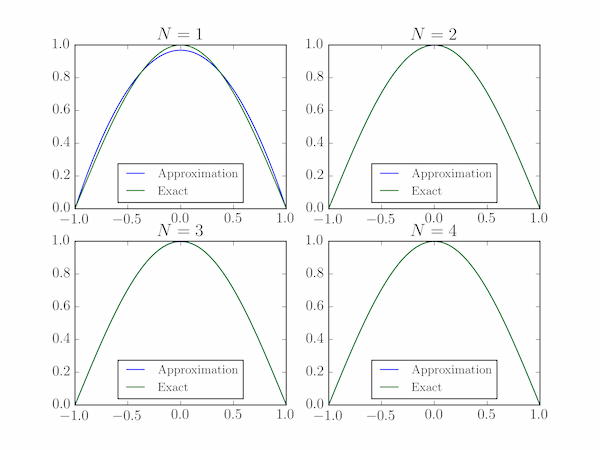
We also plot the exact and approximate wavefunctions, but they are indistinguishable for $N>1$ at this scale. The output shows good agreement of the exact and estimated energies for $N=4$:
------------------------------------------------------------
N = 1
Variational optimum E = 2.500000000000001
     Exact energy, E0 = 2.4674011002723395
------------------------------------------------------------
N = 2
Variational optimum E = 2.467437405333598
     Exact energy, E0 = 2.4674011002723395
------------------------------------------------------------
N = 3
Variational optimum E = 2.467437405329251
     Exact energy, E0 = 2.4674011002723395
------------------------------------------------------------
N = 4
Variational optimum E = 2.4674011087466323
     Exact energy, E0 = 2.4674011002723395
Note that the variational optimum is greater than the true ground state energy, as required by the variational principle.
