Solution P8.2.4
We can integrate the two coupled ordinary differential equations with scipy.integrate.odeint() and plot the results in two different ways for the two sets of parameter values, $(a,b)$.
import numpy as np
from scipy.integrate import solve_ivp
from matplotlib import pyplot as plt

fig = plt.figure()

def deriv(t, X, a, b):
    """Return the derivatives dx/dt and dy/dt."""
    x, y = X
    dxdt = a - (1+b)*x + x**2 * y
    dydt = b*x - x**2 * y
    return dxdt, dydt

x0, y0 = 1, 1

def plot_brusselator(a, b, row):
    """
    Integrate the Brusselator equations for parameters a,b and plot. """

    ti, tf = 0, 100
    soln = solve_ivp(deriv, (ti, tf), (x0, y0), dense_output=True, args=(a,b))

    t = np.linspace(ti, tf, 1000)
    X = soln.sol(t)
    ax_left = fig.add_subplot(221 + row*2)      # Lefthand axis on this row
    ax_left.plot(t, X[0], lw=1)
    ax_left.plot(t, X[1], lw=1)
    ax_left.legend((r'$x$', r'$y$'), loc='upper right')
    ax_left.set_xlabel(r'$t$')
    ax_right = fig.add_subplot(222 + row*2)      # Righthand axis on this row
    ax_right.plot(X[0], X[1], c='b', lw=1)
    ax_right.set_xlabel(r'$x$')
    ax_right.set_ylabel(r'$y$')

# Integrate and plot the Brusselator for each of the parameter pairs (1, 1.8)
# and (1, 2.02); the results from each calculation is plotted on a single row
# of the figure identified by row=0 or row=1
plot_brusselator(1, 1.8, 0)
plot_brusselator(1, 2.02, 1)

fig.tight_layout()
plt.show()
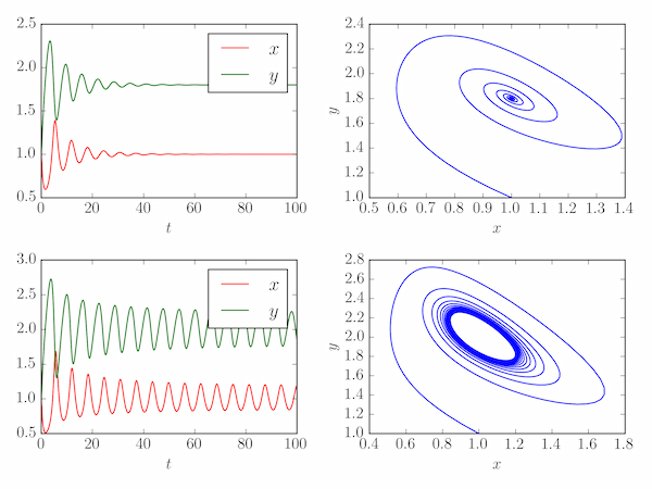
This system displays an Andronov-Hopf bifurcation at $b_\star=a^2 + 1$: for $b$ less this value (top two plots) there is a stable focus: the concentrations of X and Y converge on stable equilibrium values; for $b > b_\star$ the system enters a limit cycle (bottom two plots).