Solution P7.4.5
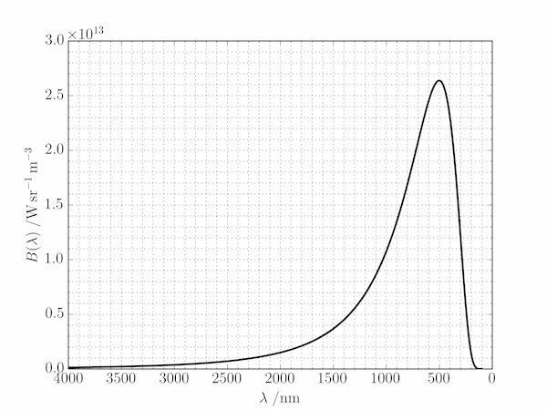
Here is one solution in monochrome with gridlines and a reversed $x$-axis.
import numpy as np
import matplotlib.pyplot as plt

# Physical constants in SI units: Planck's constant (J.s),
# the speed of light (m.s-1), Boltzmann's constant (J.K-1)
h, c, kB = 6.62606957e-34, 299792458, 1.3806488e-23
# Sun temperature, K
T = 5778

lambda_min = 100    # nm
lambda_max = 5000   # nm
n = 5000
wv = np.linspace(lambda_min, lambda_max, n)

# Planck curve as a function of wavelength in nm
B = 2 * h * c**2 / (wv*1.e-9)**5 / (np.exp(h * c / wv/1.e-9 / kB / T) - 1)

fig = plt.figure()
ax = fig.add_subplot(111)
ax.plot(wv, B, 'k', lw=2)
ax.set_xlabel(r'$\lambda\;/\mathrm{nm}$')
ax.set_ylabel(r'$B(\lambda)\;/\mathrm{W\,sr^{−1}\,m^{−3}}$')

# Wavelength decreases from left to right: 4000 nm to 0:
ax.set_xlim(left=4000, right=0)
ax.minorticks_on()
ax.grid(which='both')

plt.show()
