Question P6.5.7
Example E6.8 produced a comma-separated text file containing 10 simulations of the radioactive decay of an ensemble of 500 $\mathrm{^{14}C}$ nuclei. For each simulation column, the number of undecayed nuclei as a function of time, $N(t)$, is given; the grid of time points (in years) is in the first column.
Average the simulation data, which is available as 14C-sim.csv, and use NumPy's np.linalg.lstsq function to perform a linear least-squares fit. Retrieve the half-life of $\mathrm{^{14}C}$, $t_{1/2} = \tau\ln 2$, where:
$$
N(t) = N(0)\mathrm{e}^{-t/\tau} \quad \Rightarrow \quad \ln[N(t)] = \ln[N(0)] - \frac{t}{\tau}.
$$
Solution P6.5.7
Here is one way to fit and plot the $\mathrm{^{14}C}$ radioactive decay data.
import numpy as np
import matplotlib.pyplot as plt

# Load in the data and separate into a time column, tgrid, and columns of
# simulation runs, Nsim. Average Nsim for each time point.
arr = np.loadtxt('14C-sim.csv', delimiter=',')
tgrid = arr[:,0]
npts = len(tgrid)
Nsim = arr[:,1:]
N = Nsim.mean(axis=1)

# Least-squares fit to log(N) as a function of t: should be a straight line.
A = np.vstack((tgrid, np.ones(npts))).T
logN = np.log(N)
x, resid, _, _ = np.linalg.lstsq(A, logN, rcond=None)
m, c = x
# Our estimate of the initial number of 14C nuclei and the decay lifetime.
N0, tau = np.exp(c), -1/m
# Report N0 and the half life.
thalf = np.log(2) * tau
print(f'Fitted parameters: N0 = {N0}, half-life = {thalf:.1f} years')

# Plot the averaged data and the fit curve.
plt.plot(tgrid, N, 'x', label='Data')
plt.plot(tgrid, N0*np.exp(-tgrid/tau), label='Fit')
plt.legend()
plt.xlabel('Time, $t$ /yr')
plt.ylabel('Undecayed nuclei count, $N(t)$')
plt.savefig('ex6-5-7-decay-fit.png')
plt.show()
The resulting fitted parameters are reported as:
Fitted parameters: N0 = 511.14688017707977, half-life = 5478.0 years
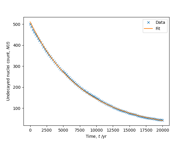
In comparison, the actual half-life is 5700 ± 40 years. The plot produced is shown below.

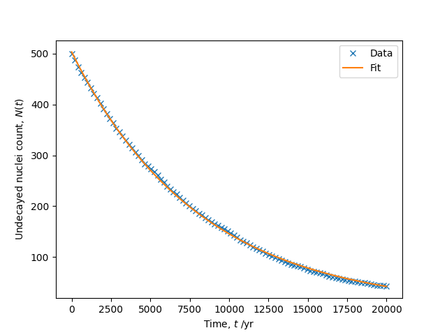
Note that although convenient and reliable, fitting a straight line to $\log(N(t))$ is not guaranteed to give the best fit parameters to $N(t)$ itself. The non-linear least squares fit (see Section 8.4.2 of the book) to the exponential function directly does a better job:
import numpy as np
from scipy.optimize import curve_fit
import matplotlib.pyplot as plt

# Load in the data and separate into a time column, tgrid, and columns of
# simulation runs, Nsim. Average Nsim for each time point.
arr = np.loadtxt('14C-sim.csv', delimiter=',')
tgrid = arr[:,0]
npts = len(tgrid)
Nsim = arr[:,1:]
N = Nsim.mean(axis=1)

# Least-squares fit to log(N) as a function of t: should be a straight line.
def decay(t, N0, tau):
    return N0 * np.exp(-t / tau)

# Initial guesses: estimate tau from the noisy data or a linear fit to log(N).
p0 = N[0], 8000
popt, pcov = curve_fit(decay, tgrid, N, p0)
N0, tau = popt

# Report N0 and the half life.
thalf = np.log(2) * tau
print(f'Fitted parameters: N0 = {N0}, half-life = {thalf:.1f} years')

# Plot the averaged data and the fit curve.
plt.plot(tgrid, N, 'x', label='Data')
plt.plot(tgrid, N0*np.exp(-tgrid/tau), label='Fit')
plt.legend()
plt.xlabel('Time, $t$ /yr')
plt.ylabel('Undecayed nuclei count, $N(t)$')
plt.savefig('ex6-5-7-decay-fit-nonlinear.png')
plt.show()
