Question P6.4.1
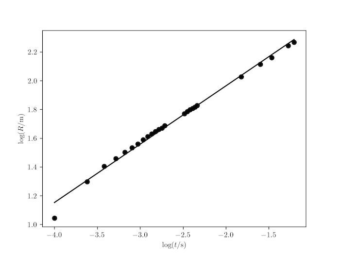
The expansion of the spherical ball of fire generated in an explosion may be analysed to deduce the initial energy, $E$, released by a nuclear weapon. The British physicist Geoffrey Taylor used dimensional analysis to demonstrate that the radius of this sphere, $R(t)$ should be related to $E$, the air density, $\rho_\mathrm{air}$, and time, $t$, through $$ R(t) = CE^{\frac{1}{5}}\rho_\mathrm{air}^{-\frac{1}{5}}t^{\frac{2}{5}}, $$ where, using model-shock wave problems, Taylor estimated the dimensionless constant $C \approx 1$. Using the data obtained from declassified timed images of the first New Mexico atomic explosion, Taylor confirmed this law and produced an estimate of the (then unknown) value of $E$. Use a log-log plot to fit the data in the table below (after G. I. Taylor, Proc. Roy. Soc. London A201, 159 (1950)) to the model and confirm the time-dependence of $R$. Taking $\rho_\mathrm{air} = 1.25\;\mathrm{kg\,m^{-3}}$ deduce $E$ and express its value in Joules and in 'kilotons of TNT' where the explosive energy released by 1 ton of TNT is arbitrarily defined to be $4.184\times 10^9\;\mathrm{J}$.
| $t\;/\mathrm{ms}$ | $R\;/\mathrm{m}$ | $t\;/\mathrm{ms}$ | $R\;/\mathrm{m}$ | $t\;/\mathrm{ms}$ | $R\;/\mathrm{m}$ |
| 0.1 | 11.1 | 1.36 | 42.8 | 4.34 | 65.6 |
| 0.24 | 19.9 | 1.50 | 44.4 | 4.61 | 67.3 |
| 0.38 | 25.4 | 1.65 | 46.0 | 15.0 | 106.5 |
| 0.52 | 28.8 | 1.79 | 46.9 | 25.0 | 130.0 |
| 0.66 | 31.9 | 1.93 | 48.7 | 34.0 | 145.0 |
| 0.80 | 34.2 | 3.26 | 59.0 | 53.0 | 175.0 |
| 0.94 | 36.3 | 3.53 | 61.1 | 62.0 | 185.0 |
| 1.08 | 38.9 | 3.80 | 62.9 | ||
| 1.22 | 41.0 | 4.07 | 64.3 |
Note: this data can be downloaded as new-mexico-blast-data.txt.
Solution P6.4.1
The code below shows a good fit to the model and predicts an energy release of 22.9 kilotons of TNT, close to the actual value of approximately 20 kilotons.
import numpy as np
import matplotlib.pyplot as plt

# Load the data, skipping the header line, and convert to log10, time in secs
t, R = np.loadtxt('new-mexico-blast-data.txt', unpack=True, skiprows=1)
logt, logR = np.log10(t/1000), np.log10(R)

# Linear, least-squares fit: logR = m(logt) + c
m, c = np.polyfit(logt, logR, 1)
print('Best fit line to log-log plot: m = {}, c = {}'.format(m,c))

# Density of air, kg.m-3
rho_air = 1.25
E = rho_air * 10**(5 * c)

# Report the estimated energy in J and kilotons of TNT (1 kton TNT = 4.184e12 J)
print('Estimated energy release: {:.3e} J, approximately = {:.1f} ktons of TNT'
            .format(E, E / 4.184e12))

# Plot the data and best fit line
plt.plot(logt, logR, 'ko')
logtfit = np.linspace(min(logt), max(logt), 1000)
lfit = m * logtfit + c
plt.plot(logtfit, lfit, 'k')
plt.show()
Output:
Best fit line to log-log plot: m = 0.40582262510045536, c = 2.7767362140219047
Estimated energy release: 9.563e+13 J, approximately = 22.9 ktons of TNT
