Question
The Gibbs phenomenon is the name given to the oscillations observed in the Fourier series of a periodic function near to a step discontinuity. For example, the square wave defined by $f(x) = 1$ for $0 < x < 1$ and $f(x) = -1$ for $1 < x < 2$ (and repeating outside the range $(0,2)$ has the Fourier series expansion: $$ f(x) = \frac{4}{\pi}\sum_{n=1,3,5,\cdots} \frac{1}{n}\sin(n\pi x) $$
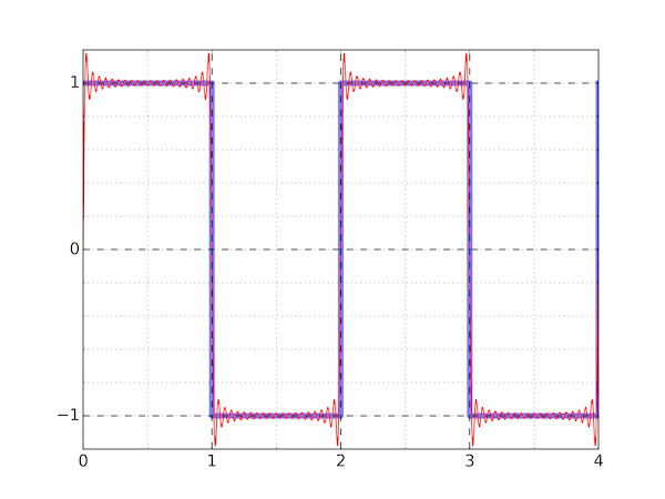
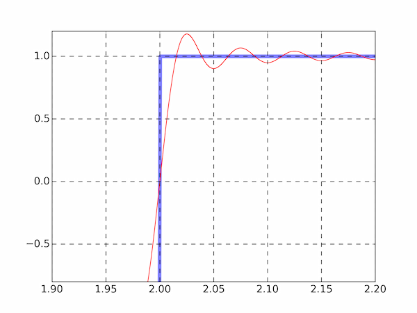
Plot $f(x)$ and its Fourier series expansion truncated at 20 terms on the same axes, (a) for $0 \le x \le 4$ and (b) zoomed in on a region exhibiting the Gibbs phenomenon.
Solution
(a) Here is one way to construct and plot the square wave and its Fourier series expansion. Recall that int rounds down in Python, so x.astype(int) % 2 is 0 for $0 \le x < 1$, 1 for $1 \le x < 2$, 0 again for $2 \le x < 3$ and so on.
The plot has been styled using some of the techniques from Chapter 7.
import numpy as np
import matplotlib.pyplot as plt

x = np.linspace(0,4,5000)

square_wave = 1 - 2 * (x.astype(int) % 2)

N = 20
fsq = np.zeros_like(x)
for i in range(N):
    n = 2*i + 1
    fsq += np.sin(n * np.pi *x) / n
fsq *= 4 / np.pi

fig, ax = plt.subplots()
ax.plot(x, square_wave, lw=5, alpha=0.5)
ax.plot(x, fsq, 'r')
ax.set_ylim(-1.2,1.2)

ax.set_xticks([0,1,2,3,4])
ax.set_xticks([0.5,1.5,2.5,3.5], minor=True)
ax.set_yticks([-1, 0, 1])
ax.set_yticks(np.arange(-1.2,1.2,0.2), minor=True)

ax.grid(b=True, c='k', lw=1, ls='--', which='major')
ax.grid(b=True, c='0.4', lw=0.5, ls=':', which='minor')

plt.show()

(b) Here are the necessary changes for plotting a zoomed-in region of the above graph. We use the default tick marks and grid lines.
fig, ax = plt.subplots()
ax.plot(x, square_wave, lw=5, alpha=0.5)
ax.plot(x, fsq, 'r')

ax.grid(b=True, c='k', lw=1, ls='--', which='major')

ax.set_ylim(-0.8,1.2)
ax.set_xlim(1.9,2.2)

plt.show()
