Solution P4.2.2
The following program produces a list of the 100 most common words in Moby Dick. The Project Gutenberg text of the novel itself is between the two identified 'marker' lines. A quick look at the this text shows that quite a few words are separated by double hyphens instead of spaces, so we replace '--' with a single space as part of the pre-processing of each line. Punctuation characters are removed next, and then the words on each line obtained by splitting the line on its whitespace.
Note the try ... except clause in used in building the wordcount dictionary: we assume that word is already a key to this dictionary and add it with a count of 1 if it isn't. This is much faster than searching the dictionary keys first to see if our word is already present in the dictionary - a good example of EAFP.
import numpy as np
import matplotlib.pyplot as plt

f =  open('moby-dick.txt', 'r', encoding='utf-8')
# Iterate over the preamble until we get to the book text
for line in f:
    if 'START OF THE PROJECT GUTENBERG EBOOK' in line:
        break

# wordcount is a dictionary of word-counts, keyed by word
wordcount = {}
for line in f:
    if 'END OF THE PROJECT GUTENBERG EBOOK' in line:
        # That's the text of the novel done: bail before the licence text, etc.
        break
    # Strip out the line endings and force everything to lower case
    line = line.strip().lower()
    # Some words are separated by --: replace this with ' '; similarly
    # remove 's (for possessives) and swap out & for and
    line = line.replace('--', ' ').replace('\'s', '').replace('&', 'and')
    # Strip any of the following punctuation
    for c in '!?":;,()\'.*[]':
        line = line.replace(c, '')

    # The line is (reasonably) clean: split it into words
    words = line.split(' ')
    for word in words:
        if not word:
            # Ignore words without any letters!
            continue
        # Update the wordcount dictionary, creating a new entry if necessary
        try:
            wordcount[word] += 1
        except KeyError:
            wordcount[word] = 1

# For a sorted list of word frequencies, create a list of (count, word) tuples
wc = []
for k,v in wordcount.items():
    wc.append((v,k))
# Sort it into decreasing order
wc.sort(reverse=True)

# Output the 100 most frequent words from the top of the wc list
for i in range(100):
    print('{:10s}: {:d}'.format(wc[i][1], wc[i][0]))

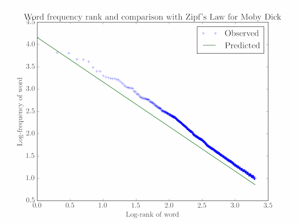
# Graphical comparison with Zipf's Law: log f(w) = log C - a log r(w)
max_rank = 2000
rank = np.linspace(1, max_rank, max_rank)
freq = np.array([ wc[i][0] for i in range(max_rank) ])
log_rank = np.log10(rank)
log_freq = np.log10(freq)
# Plot the data: log(f) against log(r)
plt.plot(log_rank, log_freq, '+', label="Observed")
# Plot the Zipf's law prediction
a, logC = 1, np.log10(freq[0])
log_zipf_freq = logC - a * log_rank
plt.plot(log_rank, log_zipf_freq, label="Predicted")
plt.xlabel('Log-rank of word')
plt.ylabel('Log-frequency of word')
plt.title("Word frequency rank and comparison with Zipf's Law for Moby Dick")
plt.legend()
plt.show()
