Solution P3.3.2
First of all, the values of $A$ and $B$ can be made more manageable by rescaling them by dividing them by Boltzmann's constant, $k_\mathrm{B} = 1.381 \times 10^{-23}\;\mathrm{J\,K^{-1}}$ — our energy scale is then measured in units of K.
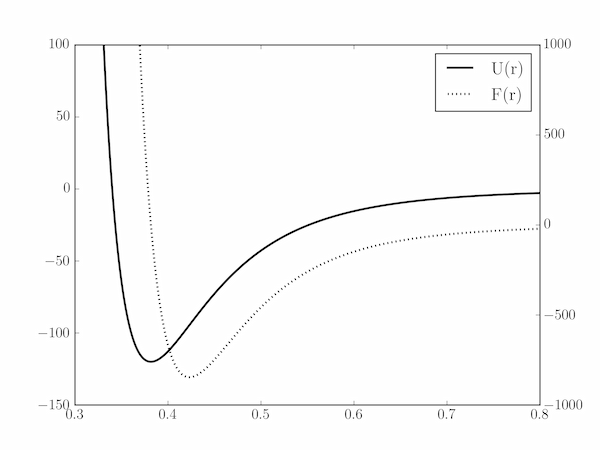
(a) The minimum in $U(r)$ occurs at $r_0 = (2B/A)^{1/6} = 0.382\;\mathrm{nm}$ (which is also where $F(r)=0$, of course); at this minimum, $\epsilon = U(r_0) = -120\;\mathrm{K}$ ($-1.657 \times 10^{-21}\;\mathrm{J}$). The potential function will increase rapidly for $r < r_0$ and somewhat less rapidly for $r > r_0$. Accordingly, we calculate it for $0.3\;\mathrm{nm} \le r \le 1\;\mathrm{nm}$, and set the y-axis limits corresponding to $-150\;\mathrm{K}\le U \le 100\;\mathrm{K}$.
For the force curve, create a twinx axis and plot $F(r)$ across the same range of $r$. The limits of our new $y$-axis can be determined in the same way as before: $F(r)$ has a minimum where $\mathrm{d}F/\mathrm{d}r = 0$ which is found to be at $r_\star = (26B/7A)^{1/6} = 0.423\;\mathrm{nm}$. This is the position of maximum attractive force between the atoms: $F(r_\star) = -845.8\;\mathrm{K\,nm^{-1}} = -1.168 \times 10^{-11}\;\mathrm{N}$. To show both regions of attractive (negative) and repulsive (positive) force, we set the ylim of the second axis to (-1000, 1000).
import numpy as np
import matplotlib.pyplot as plt

# Boltzmann's constant, J/K
kB = 1.381e-23

# The Lennard-Jones parameters:
A = 1.024e-23   # J.nm^6
B = 1.582e-26   # J.nm^12

# Adjust the units of A and B - they have more manageable values
# in K.nm^6 and K.nm^12
A, B = A / kB, B / kB

# Interatomic distance, in nm
r = np.linspace(0.3, 1, 1000)
# Interatomic potential
U = B/r**12 - A/r**6
# Interatomic force
F = 12*B/r**13 - 6*A/r**7

line1 = plt.plot(r, U, 'k', lw=2, label=r'U(r)')
plt.xlim(0.3, 0.8)
plt.ylim(-150, 100)

plt.twinx()
line2 = plt.plot(r, F, 'k', ls=':', lw=2, label=r'F(r)')
plt.xlim(0.3, 0.8)
plt.ylim(-1000, 1000)

# Jump through some hoops to get the both line's labels in the same legend:
lines = line1 + line2
labels = []
for line in lines:
    labels.append(line.get_label())
plt.legend(lines, labels)

plt.show()

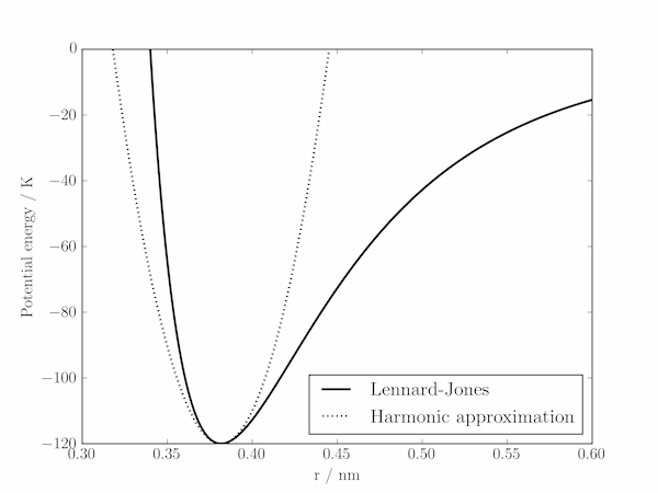
(b) With the values of $\epsilon$ and $r_0$ calculated above, it is simple to evaluate $k$ and plot $U(r)$ and $V(r)$.
import numpy as np
import matplotlib.pyplot as plt

# The Lennard-Jones parameters:
A = 1.024e-23   # J.nm^6
B = 1.582e-26   # J.nm^12

# Adjust the units of A and B - they have more manageable values
# in K.nm^6 and K.nm^12
kB = 1.381e-23  # Boltzmann's constant, J/K
A, B = A / kB, B / kB

# Interatomic distance, in nm
r = np.linspace(0.3, 1., 1000)
# Interatomic potential
U = B/r**12 - A/r**6

plt.plot(r, U, 'k', lw=2., label='Lennard-Jones')

r0 = (2*B/A)**(1./6)
epsilon = B/r0**12 - A/r0**6
k = 156*B/r0**14 - 42*A/r0**8
V = 0.5 * k * (r-r0)**2 + epsilon
plt.plot(r, V, 'k', ls=':', lw=2., label='Harmonic approximation')

plt.xlim(0.3, 0.6)
plt.ylim(-120, 0)
plt.xlabel('r / nm')
plt.ylabel('Potential energy / K')

plt.legend(loc=4)

plt.show()
