Solution P8.2.5
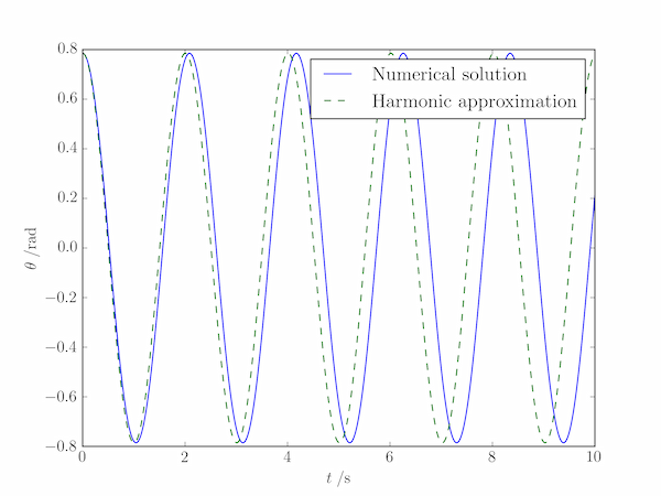
The provided second-order differential equation can, in fact, be wrangled into a single first-order differential equation but we choose here to reduce it to two such equations in variables $\theta$ and $\dot{\theta}$: \begin{align*} \frac{\mathrm{d}\dot{\theta}}{\mathrm{d}t} &= -\frac{g}{l}\sin\theta,\\ \frac{\mathrm{d}\theta}{\mathrm{d}t} &= \dot{\theta}. \end{align*}
import numpy as np
from scipy.integrate import odeint
import pylab

# Acceleration due to gravity (m.s-2), pendulum length (m)
g, l = 9.81, 1
omega = np.sqrt(g / l)
omega2 = omega**2

# Initial conditions
theta0, theta_dot0 = np.radians(45), 0
y0 = (theta0, theta_dot0)

# A suitable grid of time points
t = np.linspace(0, 10, 1000)

def deriv(y, t, omega2):
    theta, theta_dot = y
    return theta_dot, -omega2 * np.sin(theta)

# Integrate the differential equation
theta, _ = odeint(deriv, y0, t, args=(omega2,)).T

# Small angle approximation - harmonic motion
theta_harmonic = theta0 * np.cos(omega * t)

pylab.plot(t, theta, c='k', label='Numerical solution')
pylab.plot(t, theta_harmonic, c='gray',ls='--',label='Harmonic approximation')
pylab.xlabel(r'$t\;/\mathrm{s}$')
pylab.ylabel(r'$\theta\;/\mathrm{rad}$')
pylab.legend()
pylab.show()
