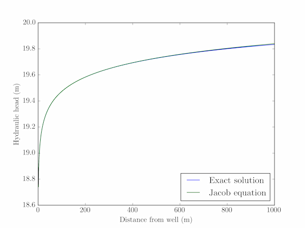
Solution P8.1.5
Here is one approach:
import numpy as np
import matplotlib.pyplot as plt
from scipy.special import exp1

Q = 1000        # Pumping rate from well (m3/day)
H0 = 20         # Initial hydraulic head (m)
S = 0.0003      # Storage coefficient
T = 1000        # Transmissivity (m2/day)

t = 1           # days
# Distance from the well (m)
r = np.linspace(0, 1000, 1000)

# Well parameter and exact solution (Theis equation) using exponential integral
u = r**2 * S / 4 / T / t
H = H0 - Q/4/np.pi/T * exp1(u)

# Approximate solution (Jacob equation) using W(u) ~ -gamma - ln u
# The Euler-Mascheroni constant (np.euler_gamma in NumPy 1.8+)
euler_gamma = 0.5772156649015329
H_jacob = H0 - Q/4/np.pi/T * np.log(np.exp(-euler_gamma)/u)

plt.plot(r,H, label='Exact solution')
plt.plot(r,H_jacob, label='Jacob equation')
plt.xlabel(r'Distance from well (m)')
plt.ylabel(r'Hydraulic head (m)')
plt.legend(loc=4)
plt.show()
This program produces the plot below
