Solution P7.2.3
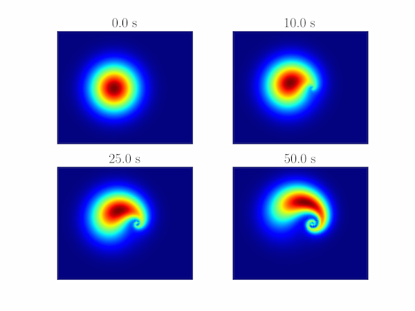
The following program produces some pleasing swirls upon advection of the initial function.
import numpy as np
import matplotlib.pyplot as plt
randint = np.random.randint

# Domain size
w = h = 10.
w = 12
# Intervals in x-, y- directions
dx = dy = 0.1
nx, ny = int(w/dx), int(h/dy)
# Time interval
dt = 0.01

# The discretized function on the domain. Note that rows (first index)
# correspond to the y-axis and columns (second index) to the x-index
u0 = np.zeros((ny, nx))
u = np.zeros((ny, nx))
x, y =  np.meshgrid(np.arange(0,nx*dx,dx), np.arange(0,ny*dy,dy))
# Initial state: a two-dimensional Gaussian function
cx, cy, alpha = 5, 5, 2
u0 = np.exp(-((x-cx)**2+(y-cy)**2)/alpha**2)

# A two-dimensional vector field discretized on our domain
cx, cy, v0 = 7, 5, 0.05
# (rx, ry) is the vector from the vortex centre to the point (x,y)
rx, ry = x - cx, y - cy
r = np.hypot(rx, ry)
# v = v0 * normalized unit vector perpendicular to r is (-ry, rx), indexed
# by row, column as (vy, vx)
v = v0 * np.dstack((rx, -ry)) / r[..., np.newaxis]
v[np.isnan(v)] = 0

def do_timestep(u0, u):
    # forward-difference in time, central-difference in space numerical
    # solution to the 2D advection equation
    u[1:-1, 1:-1] = u0[1:-1, 1:-1] - dt * (
          v[1:-1, 1:-1, 1] * (u0[1:-1, 2:] - u0[1:-1, :-2])/2/dx +  # vx.du/dx
          v[1:-1, 1:-1, 0] * (u0[2:, 1:-1] - u0[:-2, 1:-1])/2/dy)   # vy.du/dy

    u0 = u.copy()
    return u0, u

# Number of timesteps:
nsteps = 5001
# Output 4 figures at these timesteps
mfig = [0, 1000, 2500, 5000]
fignum = 0
fig = plt.figure()
for m in range(nsteps):
    u0, u = do_timestep(u0, u)
    if m in mfig:
        fignum += 1
        print(m, fignum)
        ax = fig.add_subplot(220 + fignum)
        im = ax.imshow(u.copy())
        ax.set_axis_off()
        ax.set_title('{:.1f} s'.format(m*dt))
plt.show()
