Question P6.4.2
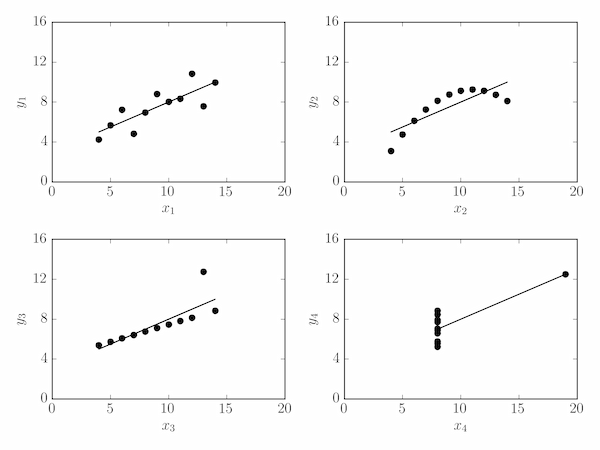
Find the mean and variance of both $x$ and $y$, the correlation coefficient and the equation of the linear regression line for each of the four data sets given in the table below. Comment on these values in the light of a plot of the data.
| $x_1$ | $y_1$ | $x_2$ | $y_2$ | $x_3$ | $y_3$ | $x_4$ | $y_4$ |
|---|---|---|---|---|---|---|---|
| 10.0 | 8.04 | 10.0 | 9.14 | 10.0 | 7.46 | 8.0 | 6.58 |
| 8.0 | 6.95 | 8.0 | 8.14 | 8.0 | 6.77 | 8.0 | 5.76 |
| 13.0 | 7.58 | 13.0 | 8.74 | 13.0 | 12.74 | 8.0 | 7.71 |
| 9.0 | 8.81 | 9.0 | 8.77 | 9.0 | 7.11 | 8.0 | 8.84 |
| 11.0 | 8.33 | 11.0 | 9.26 | 11.0 | 7.81 | 8.0 | 8.47 |
| 14.0 | 9.96 | 14.0 | 8.10 | 14.0 | 8.84 | 8.0 | 7.04 |
| 6.0 | 7.24 | 6.0 | 6.13 | 6.0 | 6.08 | 8.0 | 5.25 |
| 4.0 | 4.26 | 4.0 | 3.10 | 4.0 | 5.39 | 19.0 | 12.50 |
| 12.0 | 10.84 | 12.0 | 9.13 | 12.0 | 8.15 | 8.0 | 5.56 |
| 7.0 | 4.82 | 7.0 | 7.26 | 7.0 | 6.42 | 8.0 | 7.91 |
| 5.0 | 5.68 | 5.0 | 4.74 | 5.0 | 5.73 | 8.0 | 6.89 |
These data can be downloaded as ex6-4-a-anscombe.txt.
Solution P6.4.2
The following code calculates the required quantities.
import numpy as np
Polynomial = np.polynomial.Polynomial

# Read in the data sets and unpack into 8 rows: x1, y1, x2, ..., y4
data_sets = np.loadtxt('ex6-4-a-anscombe.txt', unpack=True)

# Loop over the data sets
for i in range(4):
    print('\nData Set #{:d}'.format(i+1), '-'*11, sep='\n')
    # Get the x,y arrays for this data set, calculate mean and variance
    x, y = data_sets[2*i], data_sets[2*i+1]
    print('x-mean = {:.2f}, x-var = {:.2f}'.format(x.mean(), x.var()))
    print('y-mean = {:.2f}, y-var = {:.2f}'.format(y.mean(), y.var()))
    # The correlation coefficient between (x, y) is the off-diagonal element
    # of the correlation coefficient matrix
    corrcoef = np.corrcoef(x, y)[0][1]
    print('(x, y) correlation coefficient = {:.3f}'.format(corrcoef))
    # Fit a straight line to the data
    pfit = Polynomial.fit(x, y, 1, window=(x.min(), x.max()))
    print('Linear regression: y = {:.2f}x + {:.2f}'.format(*pfit.coef[::-1]))
The output below shows that all four data sets have identical (or very close) values for the calculated quantities and the same linear regression equation (to 2 decimal places).
Data Set #1
-----------
x-mean = 9.00, x-var = 10.00
y-mean = 7.50, y-var = 3.75
(x, y) correlation coefficient = 0.816
Linear regression: y = 0.50x + 3.00

Data Set #2
-----------
x-mean = 9.00, x-var = 10.00
y-mean = 7.50, y-var = 3.75
(x, y) correlation coefficient = 0.816
Linear regression: y = 0.50x + 3.00

Data Set #3
-----------
x-mean = 9.00, x-var = 10.00
y-mean = 7.50, y-var = 3.75
(x, y) correlation coefficient = 0.816
Linear regression: y = 0.50x + 3.00

Data Set #4
-----------
x-mean = 9.00, x-var = 10.00
y-mean = 7.50, y-var = 3.75
(x, y) correlation coefficient = 0.817
Linear regression: y = 0.50x + 3.00
These four data sets are known as Anscombe's Quartet and demonstrate that very different underlying data sets can have the same basic statistical properties:
