Learning Scientific Programming with Python (2nd edition)
E4.19: The random-flight polymer
A simple model of a polymer in solution treats it as a sequence of randomly-oriented segments: that is, one for which there is no correlation between the orientation of one segment and any other (this is the so-called random-flight model).
We will define a class, Polymer, to describe such a polymer, in which the segment positions are held in a list of (x,y,z) tuples. A Polymer object will be initialized with the values N and a, the number of segments and the segment length respectively. The initialization method calls a make_polymer method to populate the segment positions list.
The Polymer object will also calculate the end-to-end distance, $R$, and will implement a method calc_Rg to calculate and return the polymer's radius of gyration, defined as
$$ R_\mathrm{g} = \sqrt{\frac{1}{N}\sum_{i=1}^N \left(\mathbf{r}_i - \mathbf{r}_\mathrm{CM}\right)^2} $$
import math
import random

class Polymer:
    """ A class representing a random-flight polymer in solution. """

    def __init__(self, N, a):
        """
        Initialize a Polymer object with N segments, each of length a.

        """

        self.N, self.a = N, a
        # self.xyz holds the segment position vectors as tuples
        self.xyz = [(None, None, None)] * N
        # End-to-end vector
        self.R = None
        # Make our polymer by assigning segment positions
        self.make_polymer()

    def make_polymer(self):
        """
        Calculate the segment positions, centre of mass and end-to-end
        distance for a random-flight polymer.

        """

        # Start our polymer off at the origin, (0,0,0).
        self.xyz[0] = x, y, z = cx, cy, cz = 0., 0., 0.
        for i in range(1, self.N):
            # Pick a random orientation for the next segment.
            theta = math.acos(2 * random.random() - 1)
            phi = random.random() * 2. * math.pi
            # Add on the corresponding displacement vector for this segment.
            x += self.a * math.sin(theta) * math.cos(phi)
            y += self.a * math.sin(theta) * math.sin(phi)
            z += self.a * math.cos(theta)
            # Store it, and update or centre of mass sum.
            self.xyz[i] = x, y, z
            cx, cy, cz = cx + x, cy + y, cz + z
        # Calculate the position of the centre of mass.
        cx, cy, cz = cx / self.N, cy / self.N, cz / self.N
        # The end-to-end vector is the position of the last
        # segment, since we started at the origin.
        self.R = x, y, z

        # Finally, re-centre our polymer on the centre of mass.
        for i in range(self.N):
            self.xyz[i] = self.xyz[i][0]-cx,self.xyz[i][1]-cy,self.xyz[i][2]-cz
    def calc_Rg(self):
        """
        Calculates and returns the radius of gyration, Rg. The polymer
        segment positions are already given relative to the centre of
        mass, so this is just the rms position of the segments.

        """

        self.Rg = 0.
        for x,y,z in self.xyz:
            self.Rg += x**2 + y**2 + z**2
        self.Rg = math.sqrt(self.Rg / self.N)
        return self.Rg
One way to pick the location of the next segment is to pick a random point on the surface of the unit sphere and use the corresponding pair of angles in the spherical polar coordinate system, $\theta$ and $\phi$ (where $0 \le \theta < \pi$ and $0 \le \phi < 2\pi$) to set the displacement from the previous segment's position as
$$ \begin{align*} \Delta x &= a\sin\theta\cos\phi \\ \Delta y &= a\sin\theta\sin\phi \\ \Delta z &= a\cos\theta \end{align*} $$
In the above code calculate the position of the polymer's centre of mass, $\mathbf{r}_\mathrm{CM}$, and then shift the origin of the polymer's segment coordinates so that they are measured relative to this point (that is, the segment coordinates have their origin at the polymer centre of mass).
We can test the Polymer class by importing it in the Python shell:
>>> from polymer import Polymer
>>> polymer = Polymer(1000, 0.5)   # A polymer with 1000 segments of length 0.5
>>> polymer.R           # End-to-end vector
(5.631332375722011, 9.408046667059947, -1.3047608473668109)
>>> polymer.calc_Rg()   # Radius of gyration
5.183761585363432
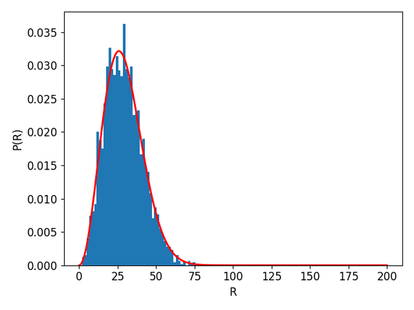
Let's now compare the distribition of the end-to-end distances with the theoretically-predicted probability density function: $$ P(R) = 4\pi R^2 \left( \frac{3}{2\pi \langle r^2 \rangle}\right)^{3/2}\exp\left(-\frac{3R^2}{2\langle r^2 \rangle}\right), $$ where the mean square position of the segments is $\langle r^2 \rangle = Na^2$
# Compare the observed distribution of end-to-end distances for Np random-
# flight polymers with the predicted probability distribution function.

import numpy as np
import matplotlib.pyplot as plt
from .polymer import Polymer
pi = np.pi

# Calculate R for Np polymers
Np = 3000
# Each polymer consists of N segments of length a
N, a = 1000, 1.
R = [None] * Np
for i in range(Np):
    polymer = Polymer(N, a)
    Rx, Ry, Rz = polymer.R
    R[i] = np.sqrt(Rx**2 + Ry**2 + Rz**2)
    # Output a progress indicator every 100 polymers
    if not (i+1) % 100:
        print(i+1)

# Plot the distribution of Rx as a normalized histogram
# using 50 bins
plt.hist(R, 50, density=1)

# Plot the theoretical probability distribution, Pr, as a function of r
r = np.linspace(0,200,1000)
msr = N * a**2
Pr = 4.*pi*r**2 * (2 * pi * msr / 3)**-1.5 * np.exp(-3*r**2 / 2 / msr)
plt.plot(r, Pr, lw=2, c='r')
plt.xlabel('R')
plt.ylabel('P(R)')
plt.show()
The program above produces a plot that typically looks like the figure below, suggesting agreement with theory.