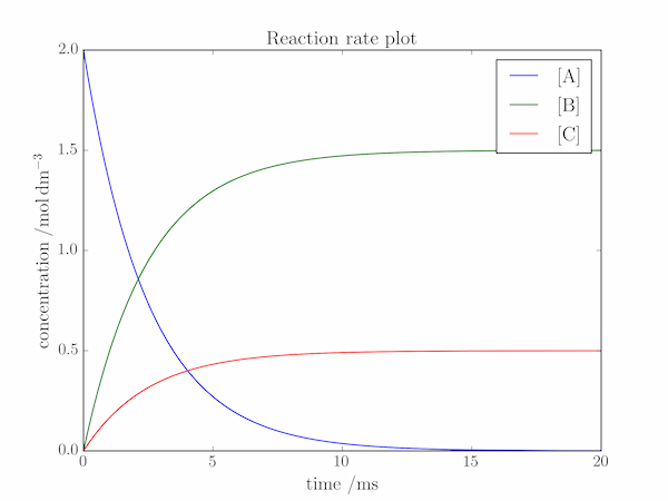
Solution P3.2.1
Here's one solution:
import pylab

k1, k2 = 300., 100. # s-1
A0 = 2. # mol.dm-3

# the time axis, in ms
t = pylab.linspace(0., 20., 1000)
A = A0 * pylab.exp(-(k1+k2)*t/1000.)
B = (k1/(k1+k2)) * (A0 - A)
C = (k2/(k1+k2)) * (A0 - A)

pylab.rc('text', usetex=True)
pylab.plot(t, A, label = '[A]')
pylab.plot(t, B, label = '[B]')
pylab.plot(t, C, label = '[C]')
pylab.xlabel('time /ms', fontsize=16.)
pylab.ylabel('$\mathrm{concentration}\;/\mathrm{mol\,dm^{-3}}$', fontsize=16.)
pylab.title('Reaction rate plot')
pylab.legend()

pylab.show()
In the above program, we define the time axis as a linspace object. The lifetime (the time taken for [A] to fall by a factor of $\mathrm{e}$) of the reactant, A, is $1/(k_1+k_2) = 2.5\;\mathrm{ms}$, so the reaction is certainly "over'' by $t = 20\;\mathrm{ms}$. The concentrations of A, B and C can be calculated using pylab's vectorized methods, and plotted with a legend as described in the text. Finally, the plot is given axis labels and a title.
