Moore's Law is the observation that the number of transistors on CPUs approximately doubles every two years. The following program illustrates this with a comparison between the actual number of transistors on high-end CPUs from between 1972 and 2012, and that predicted by Moore's Law which may be stated mathematically as: $$ n_i = n_0 2^{(y_i - y_0)/T_2}, $$ where $n_0$ is the number of transistors in some reference year, $y_0$, and $T_2 = 2$ is the number of years taken to double this number. Since the data cover 40 years, the values of $n_i$ span many orders of magnitude and it is convenient to apply Moore's Law to its logarithm, which shows a linear dependence on $y$: $$ \log_{10} n_i = \log_{10} n_0 + \frac{y_i-y_0}{T_2}\log_{10}2. $$
import pylab

# The data - lists of years:
year = [1972, 1974, 1978, 1982, 1985, 1989, 1993, 1997, 1999, 2000, 2003,
        2004, 2007, 2008, 2012]
# and number of transistors (ntrans) on CPUs in millions:
ntrans = [0.0025, 0.005, 0.029, 0.12, 0.275, 1.18, 3.1, 7.5, 24.0, 42.0,
          220.0, 592.0, 1720.0, 2046.0, 3100.0]
# turn the ntrans list into a pylab array and multiply by 1 million
ntrans = pylab.array(ntrans) * 1.e6

y0, n0 = year[0], ntrans[0]
# A linear array of years spanning the data's years
y = pylab.linspace(y0, year[-1], year[-1] - y0 + 1)
# Time taken in years for the number of transistors to double
T2 = 2.
moore = pylab.log10(n0) + (y - y0) / T2 * pylab.log10(2)

pylab.plot(year, pylab.log10(ntrans), '*', markersize=12, color='r',
           markeredgecolor='r', label='observed')
pylab.plot(y, moore, linewidth=2, color='k', linestyle='--', label='predicted')
pylab.legend(fontsize=16, loc='upper left')
pylab.xlabel('Year', fontsize=16)
pylab.ylabel('log(ntrans)', fontsize=16)
pylab.title("Moore's Law")
pylab.show()
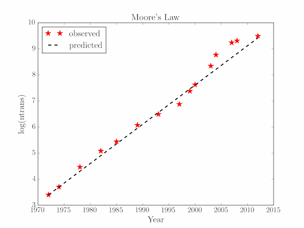
In this example, the data are given in two lists of equal length representing the year and representative number of transistors on a CPU in that year. The Moore's Law formula above is implemented in logarithmic form, using an array of years spanning the provided data. (Actually, since on a logarithmic scale this will be a straight line, really only two points are needed).
For the plot, shown below, the data are plotted as largeish stars and the Moore's Law prediction as a thick black line.