
The Storm Prediction Center (SPC) of the US National Weather Service publishes a database of tornadoes from 1950 onwards, compiled from the reports that the Weather Service's field offices submit to the publication Storm Data. Its file of tornado tracks, 1950-2025_actual_tornadoes.csv, has one row per tornado. Three of its columns are used here: the year, yr; the state, st; and the rating, mag. The rating is on the Fujita scale before 1 February 2007 and on the Enhanced Fujita scale after that date; we will treat the two as the same scale here. A rating of −9 marks a tornado rated EFU (unknown), because it caused no damage that could be surveyed.
The SPC database for 2026 is not available at the time of writing. Preliminary data for January to July 2026 in the Storm Events Database of the National Centers for Environmental Information (NCEI) list 14 intense tornadoes: 13 rated EF3 and one rated EF4 (Garfield County, Oklahoma, on 23 April).
The counts for each year and rating can be obtained with pandas, which reads the file directly from the SPC website:
import pandas as pd

URL = "https://www.spc.noaa.gov/wcm/data/1950-2025_actual_tornadoes.csv"
df = pd.read_csv(URL, usecols=["yr", "st", "mag"])
# Keep 1975-2025 and the contiguous United States.
df = df[df["yr"].between(1975, 2025) & ~df["st"].isin(["AK", "HI", "PR", "VI"])]
# One row per tornado: count the rows for each year and rating.
counts = df.groupby(["yr", "mag"]).size().unstack(fill_value=0)
intense = counts[[3, 4, 5]].sum(axis=1)
The size method counts the rows, and therefore the tornadoes, for each combination of year and rating; unstack makes a column for each rating and fills with zero the combinations that do not occur, such as a year with no EF5 tornado.
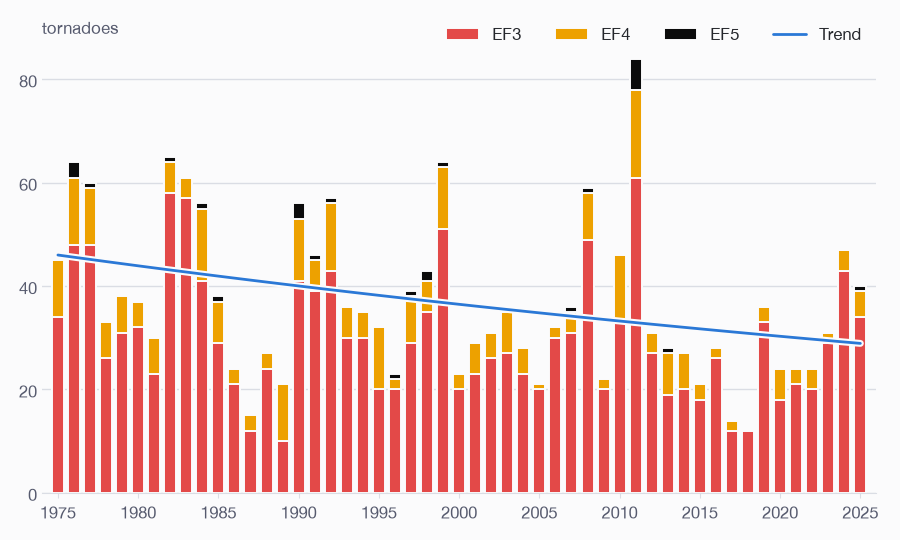
The annual counts are small whole numbers that vary widely, from 12 in 2018 to 84 in 2011. A standard model for such counts is Poisson regression, in which the count in year \(t\) has a Poisson distribution with mean \(\mu_t\), and
so that the mean count changes by a factor \(e^b\) each decade. In a Poisson distribution the variance equals the mean, but these counts are overdispersed (more variable than that): the ratio of variance to mean, estimated as the Pearson \(\chi^2\) statistic divided by its number of degrees of freedom, is 6.0. A quasi-Poisson fit keeps the Poisson estimates of \(a\) and \(b\) but multiplies their standard errors by the square root of this ratio, which widens the confidence intervals to match the scatter of the data. In statsmodels, the argument scale="X2" of the fit method can be used to do this:
import numpy as np
import statsmodels.api as sm

years = intense.index.values
X = sm.add_constant(pd.DataFrame({"decades": (years - 2000) / 10}, index=years))
fit = sm.GLM(intense, X, family=sm.families.Poisson()).fit(scale="X2")
b = fit.params["decades"]
lo, hi = fit.conf_int().loc["decades"]
print(f"Dispersion: {fit.scale:.1f}")
print(f"Change per decade: {100 * (np.exp(b) - 1):+.1f}%"
      f" (95% CI {100 * (np.exp(lo) - 1):+.1f}% to {100 * (np.exp(hi) - 1):+.1f}%),"
      f" p = {fit.pvalues['decades']:.2g}")
Dispersion: 6.0
Change per decade: -8.9% (95% CI -15.5% to -1.7%), p = 0.016
The number of intense tornadoes fell by 8.9% per decade (95% confidence interval 1.7% to 15.5%), and the fitted mean from 46 a year in 1975 to 29 a year in 2025. A negative binomial regression, another model for overdispersed counts, gives a fall of 8.7% per decade (1.9% to 15.0%).
A plain version of the figure above can be drawn with Matplotlib; the full script is given at the end of this post.
import matplotlib.pyplot as plt

fig, ax = plt.subplots()
bottom = np.zeros(len(years))
for rating, colour in zip((3, 4, 5), ("tab:red", "gold", "black")):
    ax.bar(years, counts[rating], bottom=bottom, color=colour, label=f"EF{rating}")
    bottom += counts[rating]
ax.plot(years, fit.fittedvalues, color="tab:blue", label="Trend")
ax.set_xlabel("Year")
ax.set_ylabel("Intense tornadoes")
ax.legend()
plt.show()
The number of tornadoes reported in the United States doubled between the 1950s and the 2000s, which is unlikely to have meteorological causes alone [Verbout et al., Weather and Forecasting 21, 86 (2006), doi:10.1175/WAF910.1]. Excluding the weakest tornadoes, the mean number a year has stayed roughly constant since the 1970s, but tornadoes have apparently become concentrated on fewer days, each with more of them [Brooks et al., Science 346, 349 (2014), doi:10.1126/science.1257460].
The fall in the number of intense tornadoes is statistically significant, but that in itself does not mean that intense tornadoes have become rarer. A tornado's rating is inferred from the damage it causes, so it depends on what the tornado hits and on how the damage is surveyed: the Enderlin tornado was rated EF3 for more than three months before its upgrade. Changes in damage surveys over five decades, including the move to the Enhanced Fujita scale in 2007, may account for some or all of the fall. The data show no increase in the frequency of intense tornadoes, but alone cannot be used to prove a decrease.
tornadoes_1975-2025.csv Tornadoes in the contiguous United States by year and rating, 1975–2025 (CSV)
"""Count intense tornadoes in the contiguous United States and test for a trend.

The data are the Storm Prediction Center's database of tornadoes, which has one
row per tornado. The annual counts in each rating category are fitted with a
quasi-Poisson regression on the year, and the intense tornadoes are plotted with
their trend.
"""

from pathlib import Path
from urllib.request import urlretrieve

import matplotlib.pyplot as plt
import numpy as np
import pandas as pd
import statsmodels.api as sm
from matplotlib import patheffects

SPC_URL = "https://www.spc.noaa.gov/wcm/data/1950-2025_actual_tornadoes.csv"
HERE = Path(__file__).parent
DATA_PATH = HERE / "data" / "spc" / SPC_URL.rsplit("/", 1)[1]
OUTPUT_DIR = HERE / "output"
YEAR_MIN, YEAR_MAX = 1975, 2025
# Tornadoes outside the contiguous United States.
NOT_CONTIGUOUS = ["AK", "HI", "PR", "VI"]

# Colours: EF3, EF4 and EF5 are red, yellow and black, and the trend line is blue.
PAGE = "#fbfbfc"
INK = "#24262b"
MUTED = "#565a6e"
GRID = "#dadde4"
RATING_COLOURS = {3: "#e34948", 4: "#eda100", 5: "#0b0b0b"}
TREND_COLOUR = "#2a78d6"
DPI = 100


def read_counts():
    """Return a DataFrame of tornado counts, indexed by year, one column per rating."""
    if not DATA_PATH.exists():
        DATA_PATH.parent.mkdir(parents=True, exist_ok=True)
        urlretrieve(SPC_URL, DATA_PATH)
    df = pd.read_csv(DATA_PATH, usecols=["yr", "st", "mag"])
    df = df[df["yr"].between(YEAR_MIN, YEAR_MAX) & ~df["st"].isin(NOT_CONTIGUOUS)]
    # mag is the (E)F rating, 0-5, or -9 for a tornado that could not be rated (EFU).
    counts = df.groupby(["yr", "mag"]).size().unstack(fill_value=0)
    return counts.reindex(range(YEAR_MIN, YEAR_MAX + 1), fill_value=0)


def fit_trend(years, n):
    """Fit log(mean count) = a + b * decades since 2000, as a quasi-Poisson GLM.

    The scale parameter is estimated from the Pearson chi-squared statistic, which
    widens the confidence intervals to allow for the counts' overdispersion.
    """
    X = sm.add_constant(pd.DataFrame({"decades": (years - 2000) / 10}, index=years))
    return sm.GLM(n, X, family=sm.families.Poisson()).fit(scale="X2")


def percent_per_decade(b):
    return 100 * (np.exp(b) - 1)


def style_axes(ax):
    """Light horizontal gridlines, no frame except the baseline."""
    ax.set_facecolor(PAGE)
    ax.yaxis.grid(True, color=GRID, lw=1)
    ax.set_axisbelow(True)
    for spine in ("left", "right", "top"):
        ax.spines[spine].set_visible(False)
    ax.spines["bottom"].set_color(GRID)
    ax.tick_params(axis="y", length=0, labelcolor=MUTED)
    ax.tick_params(axis="x", color=GRID, labelcolor=MUTED)
    ax.set_xticks(range(YEAR_MIN, YEAR_MAX + 1, 5))
    ax.set_xlim(YEAR_MIN - 1, YEAR_MAX + 1)


def plot_intense(counts, fit):
    """Stacked bar chart of EF3, EF4 and EF5 tornadoes with the fitted trend."""
    years = counts.index.values
    fig, ax = plt.subplots(figsize=(900 / DPI, 540 / DPI), dpi=DPI)
    fig.set_facecolor(PAGE)
    style_axes(ax)
    bottom = np.zeros(len(years))
    for rating, colour in RATING_COLOURS.items():
        ax.bar(years, counts[rating], bottom=bottom, width=0.75, color=colour,
               edgecolor=PAGE, lw=1.4, label=f"EF{rating}")
        bottom += counts[rating]
    # The fitted mean count, with a halo in the page colour over the bars.
    halo = [patheffects.Stroke(linewidth=5, foreground=PAGE), patheffects.Normal()]
    ax.plot(years, fit.fittedvalues, color=TREND_COLOUR, lw=2,
            solid_capstyle="round", path_effects=halo, label="Trend")
    ax.set_ylim(0, 90)
    ax.set_yticks(range(0, 91, 20))
    # Instead of a y-axis label, name the units beside the top gridline.
    ax.text(0, 1, "tornadoes", transform=ax.transAxes, ha="left", va="center",
            color=MUTED, backgroundcolor=PAGE)
    # Matplotlib lists lines before bars: put the trend line last.
    handles, labels = ax.get_legend_handles_labels()
    ax.legend(handles[1:] + handles[:1], labels[1:] + labels[:1], loc="upper right",
              ncols=4, frameon=False, bbox_to_anchor=(1, 1.04), labelcolor=INK)
    fig.tight_layout()
    return fig


def categories(counts):
    """Annual counts in four rating categories, for the summary of trends.

    EFU (unrated) tornadoes are counted with EF0, so that a change from one label
    to the other does not appear as a trend in either.
    """
    return {
        "EF0 or unrated": counts[0] + counts[-9],
        "EF1": counts[1],
        "EF2": counts[2],
        "EF3–EF5": counts[[3, 4, 5]].sum(axis=1),
    }


def main():
    counts = read_counts()
    years = counts.index.values
    OUTPUT_DIR.mkdir(exist_ok=True)
    table = counts.rename(columns=lambda m: "EFU" if m == -9 else f"EF{m}")
    table.index.name = "year"
    table.to_csv(OUTPUT_DIR / f"tornadoes_{YEAR_MIN}-{YEAR_MAX}.csv")

    series = {"All tornadoes": counts.sum(axis=1)} | categories(counts)
    fits = {name: fit_trend(years, n) for name, n in series.items()}
    print(f"{'Category':16s} {'dispersion':>10s} {'per decade':>10s}  95% CI            p")
    for name, fit in fits.items():
        b, (lo, hi) = fit.params["decades"], fit.conf_int().loc["decades"]
        print(f"{name:16s} {fit.scale:10.1f} {percent_per_decade(b):+9.1f}%"
              f"  [{percent_per_decade(lo):+5.1f}, {percent_per_decade(hi):+5.1f}]%"
              f"  {fit.pvalues['decades']:.2g}")

    plt.rcParams["font.family"] = ["Helvetica Neue", "Arial", "DejaVu Sans"]
    plt.rcParams["font.size"] = 12
    fig = plot_intense(counts, fits["EF3–EF5"])
    fig.savefig(OUTPUT_DIR / "intense-tornadoes.png", dpi=DPI, facecolor=PAGE)
    plt.close(fig)


if __name__ == "__main__":
    main()