Nuclear fusion cross sections and reactivities
Posted on 30 March 2021
A quick update on this blog article with some extra cross sections and an additional plot of Maxwell-averaged reactivities. The processes covered are:
$$ \begin{align*} \mathrm{D} + \mathrm{T} & \rightarrow \alpha (3.5\;\mathrm{MeV}) + n (14.1\;\mathrm{MeV}) & \\ \mathrm{D} + \mathrm{D} & \rightarrow \mathrm{T} (1.01\;\mathrm{MeV}) + p(3.02\;\mathrm{MeV})& 50\%\\ & \rightarrow \mathrm{^3He} (0.82\;\mathrm{MeV}) + n(2.45\;\mathrm{MeV}) & 50\%\\ \mathrm{D} + \mathrm{^3He} & \rightarrow \alpha (3.6\;\mathrm{MeV}) + p(14.7\;\mathrm{MeV}) & \\ \mathrm{^3He} + \mathrm{^3He} & \rightarrow 2p + \alpha + 12.86\;\mathrm{MeV} & \\ \mathrm{T} + \mathrm{^3He} & \rightarrow n + p + \alpha + 12.1\;\mathrm{MeV} & 59\% \\ & \rightarrow D (9.52\;\mathrm{MeV}) + \alpha(4.8\;\mathrm{MeV}) & 41\% \\ \mathrm{T} + \mathrm{T} & \rightarrow 2n + \alpha + 11.3\;\mathrm{MeV} & \\ p + \mathrm{^{11}B} & \rightarrow 3\alpha + 8.7\;\mathrm{MeV} & \end{align*} $$
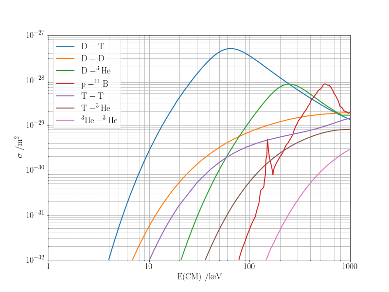
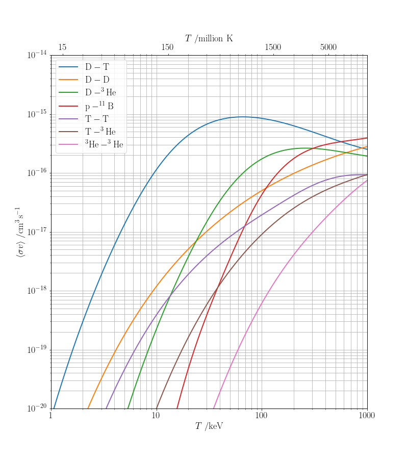
The cross section gives a probability for the reaction to occur as a function of the collision energy. In practice, the colliding particles move with a distribution of relative velocities, $f(v)$ (and hence collision energies); a useful quantity is the averaged reactivity: $$ \langle \sigma v \rangle = \int_0^\infty \sigma(v)vf(v)\,\mathrm{d}v. $$ For the Maxwell distribution of the relative speeds of the colliding particles, $$ f_\mathrm{MB}(v) = 4\pi v^2 \left(\frac{\mu}{2\pi k_\mathrm{B}T}\right)^{3/2}\exp\left(-\frac{\mu v_i^2}{2k_\mathrm{B}T}\right), $$ it can be shown [1, 2 and see below] that $$ \langle \sigma v \rangle = \frac{4}{\sqrt{2\pi\mu}}\frac{1}{(k_\mathrm{B}T)^{3/2}} \int_0^\infty \sigma(E)E\exp\left(-\frac{E}{k_\mathrm{B}T}\right)\,\mathrm{d}E, $$ where $\mu = m_1m_2/(m_1+m_2)$ is the reduced mass of the colliding particles.
The code below requires the following data files:
- D_T_-_a_n.txt
- D_D_-_T_p.txt
- D_D_-_3He_n.txt
- D_3He_-_4He_p-endf.txt
- 3He_3He_-_p_p_4He.txt
- T_3He_-_n_p_4He.txt
- T_3He_-_D_4He.txt
- T_T_-_4He_n_n.txt
- p_11B_-_3a.txt
The code:
import numpy as np
from matplotlib import rc
import matplotlib.pyplot as plt
from scipy.constants import e, k as kB
from scipy.integrate import quad
rc('font', **{'family': 'serif', 'serif': ['Computer Modern'], 'size': 18})
rc('text', usetex=True)


# To plot using centre-of-mass energies instead of lab-fixed energies, set True
COFM = True

# Reactant masses in atomic mass units (u).
u = 1.66053906660e-27
masses = {'D': 2.014, 'T': 3.016, '3He': 3.016, '11B': 11.009305167,
          'p': 1.007276466620409}

# Energy grid, 1 – 100,000 keV, evenly spaced in log-space.
Egrid = np.logspace(0, 5, 1000)

class Xsec:
    def __init__(self, m1, m2, xs):
        self.m1, self.m2, self.xs = m1, m2, xs
        self.mr = self.m1 * self.m2 / (self.m1 + self.m2)

    @classmethod
    def read_xsec(cls, filename, CM=True):
        """
        Read in cross section from filename and interpolate to energy grid.

        """

        # Read in the cross section (in barn) as a function of energy (MeV).
        E, xs = np.genfromtxt(filename, comments='#', skip_footer=2,
                              unpack=True)
        if CM:
            collider, target = filename.split('_')[:2]
            m1, m2 = masses[target], masses[collider]
            E *= m1 / (m1 + m2)

        # Interpolate the cross section onto the Egrid (keV) and
        # convert from barn to cm2.
        xs = np.interp(Egrid, E*1.e3, xs*1.e-28)
        return cls(m1, m2, xs)

    def __add__(self, other):
        return Xsec(self.m1, self.m2, self.xs + other.xs)

    def __mul__(self, n):
        return Xsec(self.m1, self.m2, n * self.xs)
    __rmul__ = __mul__

    def __getitem__(self, i):
        return self.xs[i]

    def __len__(self):
        return len(self.xs)

xs_names = {'D-T': 'D_T_-_a_n.txt',              # D + T -> α + n
            'D-D_a': 'D_D_-_T_p.txt',            # D + D -> T + p
            'D-D_b': 'D_D_-_3He_n.txt',          # D + D -> 3He + n
            'D-3He': 'D_3He_-_4He_p-endf.txt',   # D + 3He -> α + p
            'p-B': 'p_11B_-_3a.txt',             # p + 11B -> 3α
            'T-T': 'T_T_-_4He_n_n.txt',          # T + T -> 4He + 2n
            'T-3He_a': 'T_3He_-_n_p_4He.txt',    # T + 3He -> 4He + n + p
            'T-3He_b': 'T_3He_-_D_4He.txt',      # T + 3He -> 4He + D
            '3He-3He': '3He_3He_-_p_p_4He.txt',  # 3He + 3He -> 4He + 2p
           }

xs = {}
for xs_id, xs_name in xs_names.items():
    xs[xs_id] = Xsec.read_xsec(xs_name)
# Total D + D fusion cross section is due to equal contributions from the
# above two processes.
xs['D-D'] = xs['D-D_a'] + xs['D-D_b']
xs['T-3He'] = xs['T-3He_a'] + xs['T-3He_b']

def get_reactivity(xs, T):
    """Return reactivity, <sigma.v> in cm3.s-1 for temperature T in keV."""

    T = T[:, None]

    fac = 4 / np.sqrt(2 * np.pi * xs.mr * u)
    fac /= (1000 * T * e)**1.5
    fac *= (1000 * e)**2
    func = fac * xs.xs * Egrid * np.exp(-Egrid / T)
    I = np.trapz(func, Egrid, axis=1)
    # Convert from m3.s-1 to cm3.s-1
    return I * 1.e6

T = np.logspace(0, 3, 100)

xs_labels = {'D-T': '$\mathrm{D-T}$',
            'D-D': '$\mathrm{D-D}$',
            'D-3He': '$\mathrm{D-^3He}$',
            'p-B': '$\mathrm{p-^{11}B}$',
            'T-T': '$\mathrm{T-T}$',
            'T-3He': '$\mathrm{T-^3He}$',
            '3He-3He': '$\mathrm{^3He-^3He}$',
            }

DPI, FIG_WIDTH, FIG_HEIGHT = 72, 800, 900
fig = plt.figure(figsize=(FIG_WIDTH/DPI, FIG_HEIGHT/DPI), dpi=DPI)
ax = fig.add_subplot(111)

for xs_id, xs_label in xs_labels.items():
    ax.loglog(T, get_reactivity(xs[xs_id], T), label=xs_label, lw=2)
ax.legend(loc='upper left')

ax.grid(True, which='both', ls='-')
ax.set_xlim(1, 1000)
ax.set_ylim(1.e-20, 1.e-14)

xticks= np.array([1, 10, 100, 1000])
ax.set_xticks(xticks)
ax.set_xticklabels([str(x) for x in xticks])
ax.set_xlabel('$T$ /keV')
ax.set_ylabel(r'$\langle \sigma v\rangle \; /\mathrm{cm^3\,s^{-1}}$')

# A second x-axis for energies as temperatures in millions of K
ax2 = ax.twiny()
ax2.set_xscale('log')
ax2.set_xlim(1,1000)
xticks2 = np.array([15, 150, 1500, 5000])
ax2.set_xticks(xticks2 * kB/e * 1.e3)
ax2.set_xticklabels(xticks2)
ax2.set_xlabel('$T$ /million K')
plt.savefig('fusion-reactivities.png', dpi=DPI)
plt.show()

# Plot resolution (dpi) and figure size (pixels)
DPI, FIG_WIDTH, FIG_HEIGHT = 72, 800, 600
fig = plt.figure(figsize=(FIG_WIDTH/DPI, FIG_HEIGHT/DPI), dpi=DPI)
ax = fig.add_subplot(111)

for xs_id, xs_label in xs_labels.items():
    ax.loglog(Egrid, xs[xs_id], lw=2, label=xs_label)

ax.grid(True, which='both', ls='-')
ax.set_xlim(1, 1000)
xticks= np.array([1, 10, 100, 1000])
ax.set_xticks(xticks)
ax.set_xticklabels([str(x) for x in xticks])

if COFM:
    xlabel ='E(CM) /keV'
else:
    xlabel ='E /keV'
ax.set_xlabel(xlabel)

ax.set_ylabel('$\sigma\;/\mathrm{m^2}$')
ax.set_ylim(1.e-32, 1.e-27)

ax.legend(loc='upper left')
plt.savefig('fusion-xsecs2.png', dpi=DPI)
plt.show()
Derivation of reactivity
The Maxwell distribution for the relative speeds of two particles in equlibrium at temperature $T$ (in three dimensions) is: $$ f_\mathrm{MB}(v) = 4\pi v^2 \left(\frac{\mu}{2\pi k_\mathrm{B}T}\right)^{3/2}\exp\left(-\frac{\mu v_i^2}{2k_\mathrm{B}T}\right), $$ where $\mu = m_1m_2/(m_1+m_2)$ is the reduced mass of the colliding particles. Hence the reaction rate is: $$ \langle \sigma v \rangle = 4\pi \left(\frac{\mu}{2\pi k_\mathrm{B}T}\right)^{3/2} \int_0^\infty v^3\sigma(v) \exp\left(-\frac{\mu v^2}{2k_\mathrm{B}T}\right) \,\mathrm{d}v $$ To convert this integral to one over the relative kinetic energy of the particles, $E = \frac{1}{2}\mu v^2$, note that $\mathrm{d}E = \mu v \,\mathrm{d}v \Rightarrow v\,\mathrm{d}v = \mathrm{d}E / \mu$ and $v^2 = 2E/\mu$. The integral can therefore be written
$$ \begin{align*} \langle \sigma v \rangle &= 4\pi \left(\frac{\mu}{2\pi k_\mathrm{B}T}\right)^{3/2} \int_0^\infty \frac{2E}{\mu} \sigma(E) \exp\left(-\frac{E}{k_\mathrm{B}T}\right) \,\frac{\mathrm{d}E}{\mu}\\ &= \frac{4}{\sqrt{2\pi \mu}} \frac{1}{\left(k_\mathrm{B}T\right)^{3/2}} \int_0^\infty \sigma(E) E \exp\left(-\frac{E}{k_\mathrm{B}T}\right) \,\mathrm{d}E. \end{align*} $$
References
- D. D. Clayton, "Principles of Stellar Evolution and Nucleosynthesis", University of Chicago Press (1983).
- S. Atzeni and J. Meyer-ter-Vehn, "The Physics of Inertial Fusion", OUP (2004).