$k$-means clustering of exoplanet data

Posted by: christian on 26 Aug 2016

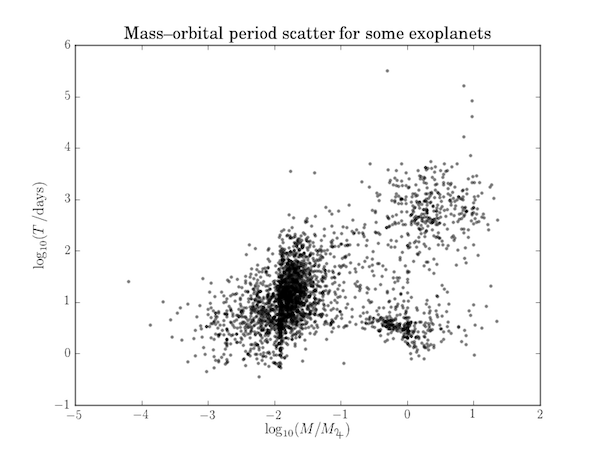
The website exoplanets.org hosts a repository of data on over 5000 exoplanets discovered by various missions and techniques. For this post, I have extracted data on the mass and orbital period of 2951 exoplanets: exoplanet-data-160824.csv. The planetary masses are expressed relative to the mass of Jupiter (M_♃) and the orbital period is in days.

Plotted below as a log-log plot, the data seem to form three clusters.

enter image description here

We can use the $k$-means algorithm, described in an example here to identify these clusters.

The code is as follows, and imports the function kmeans_pp from kmeans.py listed on the $k$-means example page.

from kmeans import kmeans_pp
import numpy as np
import matplotlib.pyplot as plt
import matplotlib

# Some matplotlib configuration: make the regular matplotlib font match the
# LaTeX font, use unicode so the en-dash (–) in the title renders properly,
# and import the wasysym package so we can use Jupiter symbol, ♃.
matplotlib.rcParams['mathtext.fontset'] = 'stix'
matplotlib.rcParams['font.family'] = 'STIXGeneral'
matplotlib.rcParams['text.usetex'] = True
matplotlib.rcParams['text.latex.unicode'] = True
matplotlib.rcParams['text.latex.preamble'] = [r'\usepackage{wasysym}']

data = np.genfromtxt('exoplanet-data-160824.csv',
                     usecols=(1,2), delimiter=',', skip_header=2)
# Filter out rows containing invalid values or values <=0 and take log10.
data = data[~np.any(np.isnan(data), axis=1)]
data = np.log10(data[np.all(data>0, axis=1)])

mu, clusters = kmeans_pp(data, 3, 5, True)
print('M / M(♃)  T / days')
print('------------------')
for row in 10**np.array(mu):
    print('{:8.4f}  {:6.2f}'.format(*row))

# Plot the clusters in distinct colours on a scatter plot.
fig, ax = plt.subplots()
colors = ['b', 'g', 'm']
for k, cluster in enumerate(clusters):
    log_mass, log_op = np.array(cluster).T
    ax.scatter(log_mass, log_op, c=colors[k], alpha=0.5, lw=0, s=10)
ax.set_xlabel(r'$\log_{10}(M/M_{\jupiter})$', fontsize=14)
ax.set_ylabel(r'$\log_{10}(T\,/\mathrm{days})$', fontsize=14)
ax.set_title('Mass–orbital period clusters for some exoplanets', fontsize=16)

plt.savefig('exoplanet-clustering.png')
plt.show()

The $k$-means clustering is repeated 5 times and the optimum clustering selected. Here is the output from one run:

iteration | this goodness | best goodness
-----------------------------------------
    1     |       66.5756 |       66.5756
    2     |       66.5756 |       66.5756
    3     |       66.5756 |       66.5756
    4     |       55.7234 |       55.7234
    5     |       55.7234 |       55.7234
M / M(♃)  T / days
------------------
  1.7233  599.72
  0.8283    4.77
  0.0139   11.54

The clusters are visualized in the following figure:

enter image description here

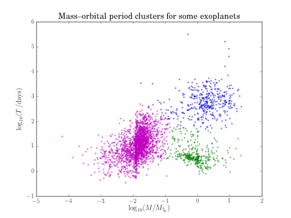
Note: These clusters are almost certainly due to observational biases and likely do not represent the true distribution of all exoplanets.

Comments

Comments are pre-moderated. Please be patient and your comment will appear soon.

There are currently no comments

$k$-means clustering of exoplanet data

Posted by: christian on 26 Aug 2016

Comments

New Comment