Fireball statistics
Posted on 15 November 2017
In astronomy, a fireball is a meteor bright enough to be seen over a wide area (either apparent magnitude greater than -4 or greater than -3 at zenith, depending on the definition used). The terms bolide and, for exceptionally bright meteors, superbolide are also used. A famous recent example is the Chelyabinsk meteor.
NASA's Center for Near Earth Object Studies maintains a database of fireball events and a reasonably fun interactive map – the Chelyabinsk meteor is the large red circle in Western Russia.
The data can be downloaded in CSV format from this page (they also expose an API) and analysed by location, energy, time, etc. The Python script below does this to demonstrate that fireballs are evenly distributed by longitude and time of day, and that the estimated radiant energy can be fit to a power law.
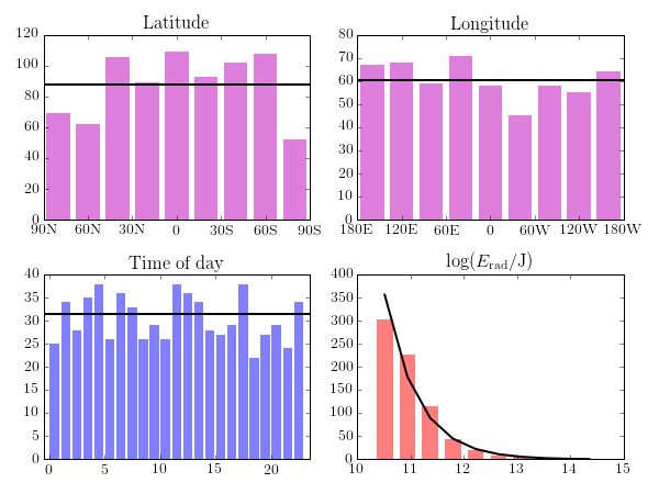
Even after accounting for the $\sin\theta$ dependence of the area element on polar angle, there seem to be more fireball events at low latitudes than near the poles. Considering the small inclinations to the ecliptic of the orbits of most objects that become meteors, this is expected (see, for example I. Halliday, Meteoritics 2, 271 (1964)).
import pandas as pd
import numpy as np
from matplotlib import rc
import matplotlib.pyplot as plt

# Use LaTeX throughout the figure for consistency
rc('font', **{'family': 'serif', 'serif': ['Computer Modern'], 'size': 14})
rc('text', usetex=True)

df = pd.read_csv('cneos_fireball_data.csv')

def convert_latitude(s):
    """Convert latitude in degrees N/S to polar angle in radians."""

    try:
        if s[-1] == 'S':
            thetap = -float(s[:-1])
        else:
            thetap = float(s[:-1])
    except TypeError:
        return np.nan
    return np.pi/2 - np.radians(thetap)

def convert_longitude(s):
    """Convert longitude in degrees E/W to azimuthal angle in radians."""

    try:
        if s[-1] == 'E':
            phi = -float(s[:-1])
        else:
            phi = float(s[:-1])
    except TypeError:
        return np.nan
    return np.radians(phi)

def convert_time(s):
    """Convert timestamp string to hours after midnight."""

    h, m, s = map(int,s[11:].split(':'))
    return h + (s/60 + m)/60

def get_bin_centres(bin_list):
    """Return the histogram bin centres given the bin edges."""
    return (bin_list[:-1] + bin_list[1:]) / 2

# Latitude: convert to polar angle in radians and discard NaNs.
theta = df['Latitude (deg.)'].apply(convert_latitude)
theta = theta[~np.isnan(theta)]
theta_bins = np.linspace(0, np.pi, 10)
theta_counts, theta_bins = np.histogram(theta, theta_bins)
theta_bins = get_bin_centres(theta_bins)

# Latitude: convert to azimuthal angle in radians and discard NaNs.
phi = df['Longitude (deg.)'].apply(convert_longitude)
phi = phi[~np.isnan(phi)]
phi_bins = np.linspace(-np.pi, np.pi, 10)
phi_counts, phi_bins = np.histogram(phi, phi_bins)
phi_bins = get_bin_centres(phi_bins)

# Time of event: convert to hours since midnight.
time = df['Peak Brightness Date/Time (UT)'].apply(convert_time)
time_bins = np.linspace(0, 23, 24)
time_counts, time_bins = np.histogram(time, time_bins)
time_bins = get_bin_centres(time_bins)

# ln(E) where E is the total radiated energy estimate.
energy = df['Total Radiated Energy (J)']
energy = np.log10(energy)
energy_counts, energy_bins = np.histogram(energy)
energy_bins = get_bin_centres(energy_bins)
# Fit a power law expression to the energy histogram.
y = np.log10(energy_counts)
mask = np.isfinite(y)
alpha, beta = np.polyfit(energy_bins[mask], y[mask], deg=1)
yfit = beta + alpha*energy_bins

# Figure dimensions and subplots; common styling parameters.
width, height, dpi = 600, 450, 72
fig, ax = plt.subplots(nrows=2, ncols=2, figsize=(width/dpi, height/dpi),
                       dpi=dpi)
bar_kwargs = {'linewidth': 0, 'alpha': 0.5, 'align': 'center'}

# Latitude histogram.
theta_bar_width = 180/len(theta_bins) * 0.8
weighted_theta = theta_counts/np.sin(theta_bins)
ax[0,0].bar(np.degrees(theta_bins), weighted_theta,
            width=theta_bar_width, color='m', **bar_kwargs)
ax[0,0].axhline(sum(weighted_theta)/len(theta_bins), c='k', lw=2)
ax[0,0].set_xticks([0, 30, 60, 90, 120, 150, 180])
ax[0,0].set_xticklabels(['90N', '60N', '30N', '0', '30S', '60S', '90S'])
ax[0,0].set_title('Latitude')

# Longitude histogram.
phi_bar_width = theta_bar_width * 2
ax[0,1].bar(np.degrees(phi_bins), phi_counts, width=phi_bar_width,
            color='m', **bar_kwargs)
ax[0,1].set_xlim(-180, 180)
ax[0,1].axhline(len(phi)/len(phi_bins), c='k', lw=2)
ax[0,1].set_xticks([-180, -120, -60, 0, 60, 120, 180])
ax[0,1].set_xticklabels(['180E', '120E', '60E', '0', '60W', '120W', '180W'])
ax[0,1].set_title('Longitude')

# Time of day histogram.
time_bar_width = 24/len(time_bins) * 0.8
ax[1,0].bar(time_bins, time_counts, width=time_bar_width,
            color='b', **bar_kwargs)
ax[1,0].set_xlim(-0.5, 23.5)
ax[1,0].axhline(len(time)/len(time_bins), c='k', lw=2)
ax[1,0].set_title('Time of day')

# Energy histogram with fitted power law.
energy_bin_width = 0.3
ax[1,1].bar(energy_bins, energy_counts, width=energy_bin_width,
            color='r', **bar_kwargs)
ax[1,1].plot(energy_bins, 10**yfit, c='k', lw=2)

ax[1,1].set_title(r'$\log(E_\mathrm{rad} / \mathrm{J})$')

plt.tight_layout()
plt.savefig('fireballs.png', dpi=dpi)