A shallow neural network for simple nonlinear classification
Posted on 18 September 2020
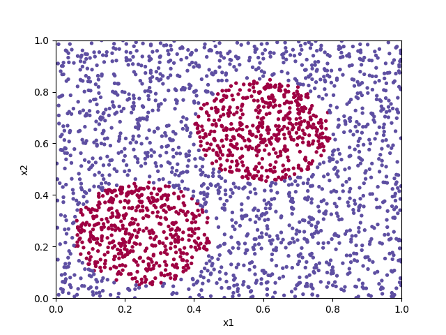
Classification problems are a broad class of machine learning applications devoted to assigning input data to a predefined category based on its features. If the boundary between the categories has a linear relationship to the input data, a simple logistic regression algorithm may do a good job. For more complex groupings, such as in classifying the points in the diagram below, a neural network can often give good results.
In a shallow neural network, the values of the feature vector of the data to be classified (the input layer) are passed to a layer of nodes (also known as neurons or units) (the hidden layer) each of which generates a response according to some activation function, $g$, acting on the weighted sum of those values, $z$. The responses of each unit in the hidden layer is then passed to a final, output layer (which may consist of a single unit), whose activation produces the classification prediction output.
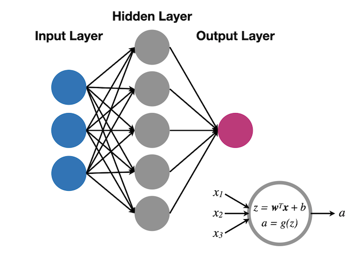
Identifying the layers with superscript labels $[0]$ (input layer), $[1]$ (hidden layer) and $[2]$ (output layer) so that $a^{[0]}_j \equiv x_j $ are the input feature values, and $a^{[2]} \equiv \hat{y}$ is the output classification we can write: $$ z^{[\ell]}_j = \sum_{k=1}^{n^{[\ell]}} w_{jk}^{[\ell]} a_k^{[\ell-1]} + b_j^{[\ell]}; \quad a^{[\ell]} = g^{[\ell]}(z^{[\ell]}_j). $$ Here, $n^{[\ell]}$ is the number of units in the $\ell$th layer; we will consider a binary classification case for which $n^{[2]} = 1$.
To train the neural network, it is presented with $m$ training examples, $\boldsymbol{x}^{(1)}, \boldsymbol{x}^{(2)}, \ldots, \boldsymbol{x}^{(m)}$ corresponding to known classifications $y^{(1)}, y^{(2)}, \ldots, y^{(m)}$ and the difference between $\hat{y}$ and $y$ (expressed in terms of some cost function) is minimized with respect to the parameters $w_{jk}^{[\ell]}$ and $b_j^{[\ell]}$ ($\ell=1,2$) as with regular logistic regression.
The $m$ column input feature vectors can be packed into a $m \times n^{[0]}$ matrix, $\boldsymbol{X}\equiv \boldsymbol{A}^{[0]}$, their classifications into a $1 \times m$ row vector, $\boldsymbol{Y}$, the unit weights into $n^{[\ell]} \times n^{[\ell-1]}$ matrices, $\boldsymbol{W}^{[\ell]}$ (for $\ell=1,2$) and the bias constants expressed as $n^{[\ell]}\times 1$ column vectors, $\boldsymbol{b}^{[\ell]}$. This allows the above equations to be implemented in matrix algebra as: $$ \begin{align*} \boldsymbol{Z}^{[1]} &= \boldsymbol{W}^{[1]}\boldsymbol{A}^{[0]} + \boldsymbol{b}^{[1]}, \quad \boldsymbol{A}^{[1]} = g^{[1]}(\boldsymbol{Z}^{[1]})\\ \boldsymbol{Z}^{[2]} &= \boldsymbol{W}^{[2]}\boldsymbol{A}^{[1]} + \boldsymbol{b}^{[2]}, \quad \boldsymbol{\hat{y}} = \boldsymbol{A}^{[2]} = g^{[2]}(\boldsymbol{Z}^{[2]}) \end{align*} $$ There are many nonlinear response functions to choose for $g^{[\ell]}$, including the logistic function, $\sigma(z) = (1+\mathrm{e}^{-z})^{-1}$, the closely-related hyperbolic tangent function, $\mathrm{tanh}$, and the rectified linear unit (ReLU) function, $x^+ = \mathrm{max}(0,x)$.
The code below implements a shallow neural network to classify the points in the file pts.txt. Progress in training the algorithm is animated by plotting the decision boundary for the set of parameters $\boldsymbol{W}^{[\ell]}$ and $\boldsymbol{b}^{[\ell]}$ at each 100th iteration of the cost function minimization.
import numpy as np
import matplotlib.pyplot as plt
import sklearn
import sklearn.linear_model

# Training rate.
alpha = 2

# Load the points and ensure shapes are X: (2, m) and Y: (1, m).
pts = np.loadtxt('pts.txt')
X, Y = pts[:,:2].T, pts[:,2][None, :]

# Number of feature vector components (should be 2!).
n0 = X.shape[0]
# Number of training examples.
m = X.shape[1]

# Number of hidden layer units.
n1 = 16
# Number of output units.
n2 = 1

# Activation function for the hidden layer: hyperbolic tan.
g1 = np.tanh
# Activation function for the output layer: logistic function.
def g2(Z):
    return 1 / (1 + np.exp(-Z))

def predictions(X, W1, b1, W2, b2):
    """
    Return the predictions, A2 (and various intermediate quantities for
    caching) for the parameters W1, b1, W2, b2 on the input matrix, X.
    """

    Z1 = W1 @ X + b1
    A1 = g1(Z1)
    Z2 = W2 @ A1 + b2
    A2 = g2(Z2)
    return Z1, A1, Z2, A2

def cost(Yhat, Y):
    """Evaluate and return the cost function J(Yhat, Y)."""
    return -np.sum(Y * np.log(Yhat) + (1 - Y) * np.log(1 - Yhat)) / m

def backprop(A1, Z1, A2, Z2, W1, b1, W2, b2):
    """Backpropagation to update the fit parameters."""

    # The derivatives of the cost function with respect to the various
    # quantities, dJ/dQ are assigned to variables named dQ.

    # For g2 = sigmoid logistic function.
    dZ2 = A2 - Y
    dW2 = dZ2 @ A1.T / m
    db2 = np.sum(dZ2, axis=1, keepdims=True) / m
    # For g1 = tanh activation function.
    dZ1 = W2.T @ dZ2 * (1 - A1**2)
    dW1 = dZ1 @ X.T / m
    db1 = np.sum(dZ1, axis=1, keepdims=True) / m

    W1 -= alpha * dW1
    b1 -= alpha * db1
    W2 -= alpha * dW2
    b2 -= alpha * db2
    return W1, b1, W2, b2

def initialize_params():
    """Randomly initialize the W coefficients, initialize the biases to zero."""
    W1 = np.random.randn(n1, n0) * 0.01
    b1 = np.zeros((n1, 1))
    W2 = np.random.randn(n2, n1) * 0.01
    b2 = np.zeros((n2, 1))
    return W1, b1, W2, b2

def plot_decision_boundary(X, y, params):
    """Plot the decision boundary for prediction trained on X, y."""

    # Set min and max values and give it some padding.
    x_min, x_max = X[0, :].min() - 0.1, X[0, :].max() + 0.1
    y_min, y_max = X[1, :].min() - 0.1, X[1, :].max() + 0.1
    h = 0.01
    # Generate a meshgrid of points with orthogonal spacing.
    xx, yy = np.meshgrid(np.arange(x_min, x_max, h), np.arange(y_min, y_max, h))
    # Prediction of the classified values across the whole grid.
    Z = np.round(predictions(np.c_[xx.ravel(), yy.ravel()].T, *params)[-1])
    Z = Z.reshape(xx.shape)
    # Plot the decision boundary as a contour plot and training examples.
    plt.contourf(xx, yy, Z, cmap=plt.cm.Spectral)
    plt.scatter(X[0, :], X[1, :], c=y, cmap=plt.cm.Spectral, s=8)
    plt.ylabel('x2')
    plt.xlabel('x1')

def train(X, Y, max_it=1000):
    """Train the neural network on the features X classified as Y."""

    W1, b1, W2, b2 = initialize_params()

    for it in range(max_it):
        Z1, A1, Z2, A2 = predictions(X, W1, b1, W2, b2)
        J = cost(A2, Y)
        W1, b1, W2, b2 = backprop(A1, Z1, A2, Z2, W1, b1, W2, b2)
        if not it % 100:
            # Provide an update on the progress we have made so far.
            print('{}: J = {}'.format(it, J))
            # Clear the current figure and redraw with the latest prediction.
            plt.clf()
            plot_decision_boundary(X, Y, (W1, b1, W2, b2))
            plt.xlim(0,1)
            plt.ylim(0,1)
            plt.savefig('frames/{:05d}.png'.format(it))

    return W1, b1, W2, b2

W1, b1, W2, b2 = train(X, Y, 7000)

plot_decision_boundary(X, Y, (W1, b1, W2, b2))
plt.xlim(0,1)
plt.ylim(0,1)
plt.show()
The frames of the animation are saved as PNG image files to the directory frames/ and can be turned into an animated GIF with, e.g. ImageMagick's convert utility.