Plotting the decision boundary of a logistic regression model
Posted on 17 September 2020
In the notation of this previous post, a logistic regression binary classification model takes an input feature vector, $\boldsymbol{x}$, and returns a probability, $\hat{y}$, that $\boldsymbol{x}$ belongs to a particular class: $\hat{y} = P(y=1|\boldsymbol{x})$. The model is trained on a set of provided example feature vectors, $\boldsymbol{x}^{(i)}$, and their classifications, $y^{(i)} = 0$ or $1$, by finding the set of parameters that minimize the difference between $\hat{y}^{(i)}$ and $y^{(i)}$ in some sense.
These model parameters are the components of a vector, $\boldsymbol{w}$ and a constant, $b$, which relate a given input feature vector to the predicted logit or log-odds, $z$, associated with $\boldsymbol{x}$ belonging to the class $y=1$ through $$ z = \boldsymbol{w}^T\boldsymbol{x} + b. $$ In this formulation, $$ z = \ln \frac{\hat{y}}{1-\hat{y}} \quad \Rightarrow \hat{y} = \sigma(z) = \frac{1}{1+\mathrm{e}^{-z}}. $$ Note that the relation between $z$ and the components of the feature vector, $x_j$, is linear. In particular, for a two-dimensional problem, $$ z = w_1x_1 + w_2x_2 + b. $$ It is sometimes useful to be able to visualize the boundary line dividing the input space in which points are classified as belonging to the class of interest, $y=1$, from that space in which points do not. This could be achieved by calculating the prediction associated with $\hat{y}$ for a mesh of $(x_1, x_2)$ points and plotting a contour plot (see e.g. this scikit-learn example).
Alternatively, one can think of the decision boundary as the line $x_2 = mx_1 + c$, being defined by points for which $\hat{y}=0.5$ and hence $z=0$. For $x_1 = 0$ we have $x_2=c$ (the intercept) and
$$
0 = 0 + w_2x_2 + b \quad \Rightarrow c = -\frac{b}{w_2}.
$$
For the gradient, $m$, consider two distinct points on the decision boundary, $(x_1^a,x_2^a)$ and $(x_1^b,x_2^b)$, so that $m = (x_2^b-x_2^a)/(x_1^b-x_1^a)$. Along the boundary line,
$$
\begin{align*}
& 0 = w_1x_1^b + w_2x_2^b + b - (w_1x_1^a + w_2x_2^a + b)\\
\Rightarrow & -w_2(x_2^b - x_2^a) = w_1(x_1^b - x_1^a)\\
\Rightarrow & m = -\frac{w_1}{w_2}.
\end{align*}
$$
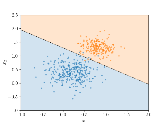
To see this in action, consider the data in linpts.txt, which maybe classified using scikit-learn's LogisticRegression classifier. The following script retrieves the decision boundary as above to generate the following visualization.
import numpy as np
import matplotlib.pyplot as plt
import sklearn.linear_model
plt.rc('text', usetex=True)

pts = np.loadtxt('linpts.txt')
X = pts[:,:2]
Y = pts[:,2].astype('int')

# Fit the data to a logistic regression model.
clf = sklearn.linear_model.LogisticRegression()
clf.fit(X, Y)

# Retrieve the model parameters.
b = clf.intercept_[0]
w1, w2 = clf.coef_.T
# Calculate the intercept and gradient of the decision boundary.
c = -b/w2
m = -w1/w2

# Plot the data and the classification with the decision boundary.
xmin, xmax = -1, 2
ymin, ymax = -1, 2.5
xd = np.array([xmin, xmax])
yd = m*xd + c
plt.plot(xd, yd, 'k', lw=1, ls='--')
plt.fill_between(xd, yd, ymin, color='tab:blue', alpha=0.2)
plt.fill_between(xd, yd, ymax, color='tab:orange', alpha=0.2)

plt.scatter(*X[Y==0].T, s=8, alpha=0.5)
plt.scatter(*X[Y==1].T, s=8, alpha=0.5)
plt.xlim(xmin, xmax)
plt.ylim(ymin, ymax)
plt.ylabel(r'$x_2$')
plt.xlabel(r'$x_1$')

plt.show()