Blog
A blog of Python-related topics and code.
-
Simulating foraminifera
Posted on 07 December 2015
-
The Lorenz attractor
Posted on 04 December 2015
-
The moment of inertia of a random flight polymer
Posted on 04 November 2015
-
Counting seeds with Python
Posted on 21 September 2015
-
Penrose Tiling 2: Implementation and Examples
Posted by christian on 26 May 2015
-
Penrose Tiling 1: Introduction
Posted by christian on 15 May 2015
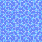
This blog post introduces Penrose tiling, a type of aperiodic tiling discovered by mathematician Roger Penrose in the 1970s. Penrose tilings are constructed using specific shapes (tiles) that can cover a plane without repeating patterns. The post focuses on the P3 tiling scheme, which uses two rhombus-shaped tiles derived from Robinson triangles with side ratios related to the Golden Ratio ($ϕ$) and its inverse ($ψ$).
-
Parenthesis matching in Python
Posted on 04 May 2015