Posted by: christian on 3 Sep 2020
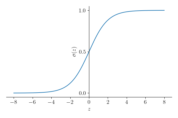
Simple logistic regression is a statistical method that can be used for binary classification problems. In the context of image processing, this could mean identifying whether a given image belongs to a particular class ($y=1$) or not ($y=0$), e.g. "cat" or "not cat". A logistic regression algorithm takes as its input a feature vector $\boldsymbol{x}$ and outputs a probability, $\hat{y} = P(y=1|\boldsymbol{x})$, that the feature vector represents an object belonging to the class. For images, the feature vector might be just the values of the red, green and blue (RGB) channels for each pixel in the image: a one-dimensional array of $n_x = n_\mathrm{height} \times n_\mathrm{width} \times 3$ real numbers formed by flattening the three-dimensional array of pixel RGB values. A logistic regression model is so named because it calculates $\hat{y} = \sigma(z)$ where $$ \sigma(z) = \frac{1}{1+\mathrm{e}^{-z}} $$ is the logistic function and $$ z = \boldsymbol{w}^T\boldsymbol{x} + b, $$ for a set of parameters, $\boldsymbol{w}$ and $b$. $\boldsymbol{w}$ is a $n_x$-dimensional vector (one component for each component of the feature vector) and b is a constant "bias".
Training a logistic regression algorithm involves obtaining the optimum values of $\boldsymbol{w}$ and $b$ such that $\hat{y}^{(i)}$ most closely predicts $y^{(i)}$ for a set of $m$ provided, pre-classified examples (i.e. $m$ images corresponding to feature vectors $\boldsymbol{x}^{(i)}$ for which the classification $y^{(i)}$ is known): this is a supervised learning technique. In practice, this usually means calculating the loss function, $$ \mathcal{L}(\hat{y}^{(i)}, y^{(i)})) = -[y^{(i)}\log \hat{y}^{(i)} + (1 - y^{(i)})\log(1-\hat{y}^{(i)})] $$ for each training example, $i$, and minimizing the cost function, $$ J(\boldsymbol{w}, b) = \frac{1}{m}\sum_{i=1}^m \mathcal{L}(\hat{y}^{(i)}, y^{(i)})) $$ across all $m$ training examples. The loss function captures, in a way suitable for numerical minimization of $J$, the difference between the predicted and actual classification of each training example. It can be shown that $$ \frac{\partial\mathcal{L}}{\partial w_j} = (\hat{y}^{(i)} - y^{(i)})x_j^{(i)}\quad\mathrm{and}\quad \frac{\partial\mathcal{L}}{\partial b} = \hat{y}^{(i)} - y^{(i)}, $$ where $j=1,2,\ldots,n_x$ labels the components of the feature vector.
In numerically minimizing $J(\boldsymbol{w}, b)$ one starts with an initial guess for $w_j$ and $b$ and uses these expressions to determine how to change them iteratively so that $J$ keeps decreasing. That is, on each iteration the values of the parameters are changed according to descent along the steepest gradient: $$ w_j \rightarrow w_j - \alpha \frac{\partial J}{\partial w_j} = w_j - \frac{\alpha}{m}\sum_{i=1}^m \frac{\partial\mathcal{L}}{\partial w_j}, $$ and similarly for $b$, where $\alpha$ is some learning rate that determines how large each step taken in the direction of greatest decrease in $J$ is. Choosing a suitable value for $\alpha$ is a subtle art (too small and the training is slow, too large and the steps taken in gradient descent are too large and the training may not converge reliably on the minimum in $J$), but for small, simple problems can be determined by trial-and-error.
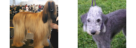
The following script trains this simple model to discriminate between pictures of Afghan Hounds and Bedlington Terriers (a fairly sympathetic task, given the dogs have quite different colours). The training and test data are provided as HDF5 files and have been obtained by cropping and resizing images from the Stanford Dogs Dataset. Here is one image from each class:
import numpy as np
import h5py
# Training rate
alpha = 0.002
def sigmoid(z):
"""Return the logistic function sigma(z) = 1/(1+exp(-z))."""
return 1 / (1+np.exp(-z))
def cost(Y, Yhat):
"""Return the cost function for predictions Yhat of classifications Y."""
return (- Y @ np.log(Yhat.T) - (1 - Y) @ np.log(1 - Yhat.T)) / m
def accuracy(Y, Yhat):
"""Return measure of the accuracy with which Yhat predicts Y."""
return 1 - np.mean(np.abs(Y - Yhat.round()))
def model(X, w, b):
"""Apply the logistic model parameterized by w, b to features X."""
z = w.T @ X + b
Yhat = sigmoid(z)
return z, Yhat
def train(X, Y, max_it=1000):
"""Train the logistic regression algorithm on the data X classified as Y."""
# Parameter vector, w, and constant term (bias), b.
# For random initialization, use the following:
#w, b = np.random.random((nx,1)) * 0.01, 0.01
# To initialize with zeros, use this line instead:
w, b = np.zeros((nx,1)), 0
def propagate(w, b):
"""Propagate the training by advancing w, b to reduce the cost, J."""
z, Yhat = model(X, w, b)
w -= alpha / m * (X @ (Yhat - Y).T)
b -= alpha / m * np.sum(Yhat - Y)
J = np.squeeze(cost(Y, Yhat))
if not it % 100:
# Provide an update on the progress we have made so far.
print('{}: J = {}'.format(it, J))
print('train accuracy = {:g}%'.format(accuracy(Y, Yhat) * 100))
return w, b
# Train the model by iteratively improving w, b.
for it in range(max_it):
w, b = propagate(w, b)
return w, b
# Our training data, in an HDF5 file.
ds_train = h5py.File('dogs_train.h5', 'r')
# Normalise the pixel data (RGB channels) to be in the range 0-1.
ds_x = np.array(ds_train["dogs_train_x"]).T / 255
ds_y = np.array(ds_train["dogs_train_y"])
# Number of training examples.
m = len(ds_y)
# Dimension of the feature vector for each example.
nx = ds_x.size // m
# Packed feature vector and associated classification.
X, Y = ds_x.reshape((nx, m)), ds_y.reshape((1, m))
# Train the model
w, b = train(X, Y)
# Now the test data
ds_test = h5py.File('dogs_test.h5', 'r')
ds_x = np.array(ds_test["dogs_test_x"]).T / 255
ds_y = np.array(ds_test["dogs_test_y"])
# Number of test examples.
m = len(ds_y)
# Dimension of the feature vector for each example.
nx = ds_x.size // m
# Packed feature vector and associated classification.
X, Y = ds_x.reshape((nx, m)), ds_y.reshape((1,m))
z, Yhat = model(X, w, b)
print('test accuracy = {}%'.format(accuracy(Y, Yhat) * 100))
#import sys; sys.exit()
from PIL import Image
def categorize_image(filename):
"""Categorize the image provided in filename.
Return 1 if the image is categorized in the y=1 class and otherwise 0.
"""
im = Image.open(filename)
ds_x = np.asarray(im, dtype='uint8')[:, :, :3].T / 255
ds_y = np.array([1])
# Number of test examples.
m = len(ds_y)
# Dimension of the feature vector for each example.
nx = ds_x.size // m
# Packed feature vector and associated classification.
X, Y = ds_x.reshape((nx, m)), ds_y.reshape((1,m))
z, Yhat = model(X, w, b)
return np.squeeze(Yhat) > 0.5
def report_category(filename, predictedY):
s = 'a Bedlington Terrier' if predictedY else 'an Afghan Hound'
print(filename, 'is ' + s)
filename = 'afghan.png'
report_category(filename, categorize_image(filename))
filename = 'bedlington.png'
report_category(filename, categorize_image(filename))
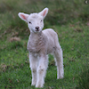
filename = 'lamb.png'
report_category(filename, categorize_image(filename))
The output indicates a reasonable model which discriminates between the two dog breeds 82% of the time on the test data:
0: J = 0.6931471805599454
train accuracy = 49.3976%
100: J = 0.40646680736736357
train accuracy = 83.9357%
200: J = 0.30963910029260394
train accuracy = 92.7711%
300: J = 0.27044432864585155
train accuracy = 93.1727%
400: J = 0.2403748716897039
train accuracy = 94.7791%
500: J = 0.21618082409768039
train accuracy = 96.3855%
600: J = 0.1961962194683076
train accuracy = 96.7871%
700: J = 0.17939225598255604
train accuracy = 97.1888%
800: J = 0.16506777147246057
train accuracy = 97.5904%
900: J = 0.1527192203531857
train accuracy = 97.5904%
test accuracy = 82.35294117647058%
afghan.png is an Afghan Hound
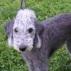
bedlington.png is a Bedlington Terrier
lamb.png is a Bedlington Terrier
The further test images used are an Afghan (correctly classified), a Bedlington Terrier (correctly classified), and a lamb that gets classified as a Bedlington Terrier.
Share on Twitter Share on Facebook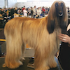
Comments
Comments are pre-moderated. Please be patient and your comment will appear soon.
Elie RAPHAEL 3 years, 7 months ago
Thanks a lot Christian for this great website!
Link | ReplyRegarding your last blog (Logistic regression for image classification), could you please indicate how to download the training and test data? Thanks.
Have a great day,
Elie.
christian 3 years, 7 months ago
Hi Elie,
Link | ReplyI'm glad you find it interesting – the training and test data are available as compressed HDF5 files from the links in the paragraph above the code: dogs_train.h5.gz and dogs_test.h5.gz (they need to be (g)unzipped first).
Cheers, Christian
Sandip 2 years, 1 month ago
Hi Christian,
Link | ReplyI have collection of images of two classes. And I am looking for binary image classification.
I am looking for help on how to create dataset from these images so that I can use it for your given model.
christian 2 years, 1 month ago
Usually it is helpful for the images to have the same dimensions. In this respect, the following might help you: https://scipython.com/blog/cropping-a-square-region-from-an-image/. It's been a while, but I think I cropped the images for this article from the Stanford Dogs Dataset by hand using this script.
Link | ReplyNew Comment