P9.2.5The line spectrum of carbon dioxide
The HITRAN database provides a list of molecular line intensities for modeling radiative transmission in planetary atmospheres. Its native format consists of 160-character records of fixed-width fields.
Use pandas to read in the file CO2-transitions.par. This text file contains fixed-width fields; the relevant fields are in character columns 4 – 15 (wavenumber, \(\tilde{\nu}\), in \(\mathrm{cm^{-1}}\)) and columns 16 – 25 (spectral line intensity, \(S\), at 296 K in \(\mathrm{cm^{-1}/(molecule\,cm^{-2})}\), weighted by isotopologue abundance). Note: these column numbers are indexed starting at 1.
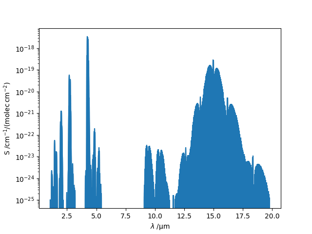
Plot line intensity against wavelength for these transitions in the infrared region of the spectrum (\(\lambda\) = 1 μm to 20 μm, corresponding to wavenumber \(\tilde{\nu} = 500\;\mathrm{cm^{-1}}\) to \(10\,000\;\mathrm{cm^{-1}}\)), where carbon dioxide (\(\mathrm{CO_2}\)) is responsible for a significant fraction of the greenhouse effect in Earth's atmosphere.
Hint: Use Matplotlib's stem plotting function.
Show solution
Here is one approach:
import pandas as pd
import matplotlib.pyplot as plt

df = pd.read_fwf(
    "CO2-transitions.par",
    colspecs=[(3, 15), (15, 25)],
    header=None,
    names=["nu", "S"],
)
df["lambda /um"] = 1.0e4 / df["nu"]

fig, ax = plt.subplots()
ax.stem(df["lambda /um"], df["S"], markerfmt="none")
ax.set_yscale("log")
ax.set_xlabel(r"$\lambda\;/\mathrm{\mu m}$")
ax.set_ylabel(r"S /$\mathrm{cm^{-1}/(molec\,cm^{-2})}$")
plt.show()