The Theis equation · scipython.com

P8.1.5The Theis equation

The drawdown or change in hydraulic head, $$s$$ (a measure of the water pressure above some geodetic datum) a distance $$r$$ from a well at time $$t$$ from which water is being pumped at a constant rate, $$Q$$ , can be modelled using the Theis equation,

s(r, t) = H_0 - H(r,t) = \frac{Q}{4\pi T}W(u), \quad \mathrm{where}\quad u = \frac{r^2S}{4Tt}.

Here $$H_0$$ is the hydraulic head in the absence of the well, $$S$$ is the aquifer storage coefficient (volume of water released per unit decrease in $$H$$ per unit area) and $$T$$ is the transmissivity (a measure of how much water is transported horizontally per unit time). The Well Function, $$W(u)$$ is simply the exponential integral, $$E_1(u)$$ .

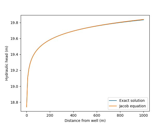
For a well being pumped at $Q = 1000\;\mathrm{m^3\,day^{-1}}$ from an aquifer described by the parameters $H_0 = 20\;\mathrm{m}$ , $$S = 0.0003$$ , $T = 1000\;\mathrm{m^2\,day^{-1}}$ , determine the height of the hydraulic head as a function of $$r$$ after $t = 1\;\mathrm{day}$ of pumping.

Compare your answer with the approximate version of the Theis equation known as the Jacob equation, in which the well function is taken to be appoximately $W(u) \approx -\gamma - \ln u$ where $\gamma=0.577215664\cdots$ is the Euler-Mascheroni constant.

Show solution

Here is one approach:

theisequation

import numpy as np
import matplotlib.pyplot as plt
from scipy.special import exp1

Q = 1000  # Pumping rate from well (m3/day)
H0 = 20  # Initial hydraulic head (m)
S = 0.0003  # Storage coefficient
T = 1000  # Transmissivity (m2/day)

t = 1  # days
# Distance from the well (m): 10 metre intervals out to 1 km.
r = np.arange(0, 1001, 10)
# NB we can't allow r = 0 m (singularity in solution).
r[0] = 1

# Well parameter and exact solution (Theis equation) using exponential integral
u = r**2 * S / 4 / T / t
H = H0 - Q / 4 / np.pi / T * exp1(u)

# Approximate solution (Jacob equation) using W(u) ~ -gamma - ln u
H_jacob = H0 - Q / 4 / np.pi / T * np.log(np.exp(-np.euler_gamma) / u)

plt.plot(r, H, label="Exact solution")
plt.plot(r, H_jacob, label="Jacob equation")
plt.xlabel("Distance from well (m)")
plt.ylabel("Hydraulic head (m)")
plt.legend(loc=4)
plt.show()

This program produces the plot below

Exact and approximate solution to the Theis equation.