A quantum particle in a gravitational field

Consider a particle of mass $$m$$ moving in a constant gravitational field such that its potential energy at a height $$z$$ above a surface is $$mgz$$ . If the particle bounces elastically on the surface, the classical probability density corresponding to its position is

P_\mathrm{cl}(z) = \frac{1}{\sqrt{z_\mathrm{max}(z_\mathrm{max}-z)}},

where $z_\mathrm{max}$ is the maximum height it reaches.

The quantum mechanical behaviour of this system may described by the solution to the time-independent Schrödinger equation,

-\frac{\hbar^2}{2m}\frac{\mathrm{d}^2\psi}{\mathrm{d}z^2} + mgz\psi = E\psi

which is simplified by the coordinate rescaling $q = z/\alpha$ where $\alpha =(\hbar^2 / 2m^2g)^{1/3}$ :

\frac{\mathrm{d}^2\psi}{\mathrm{d}q^2} - (q-q_E)\psi = 0, \quad \mathrm{where}\; q_E = \frac{E}{mg\alpha}.

The solutions to this differential equation are the Airy functions. The boundary condition $\psi(z)\rightarrow 0$ as $z\rightarrow \infty$ specifically gives:

\psi(q) = N_E\mathrm{Ai}(q-q_E),

where $$N_E$$ is a normalization constant.

The second boundary condition, $\psi(q=0) = 0$ , leads to quantization in terms of a quantum number $n=1,2,3,\cdots$ , with scaled energy values $$q_E$$ found from the zeros of the Airy function: $\mathrm{Ai}(-q_E) = 0$ .

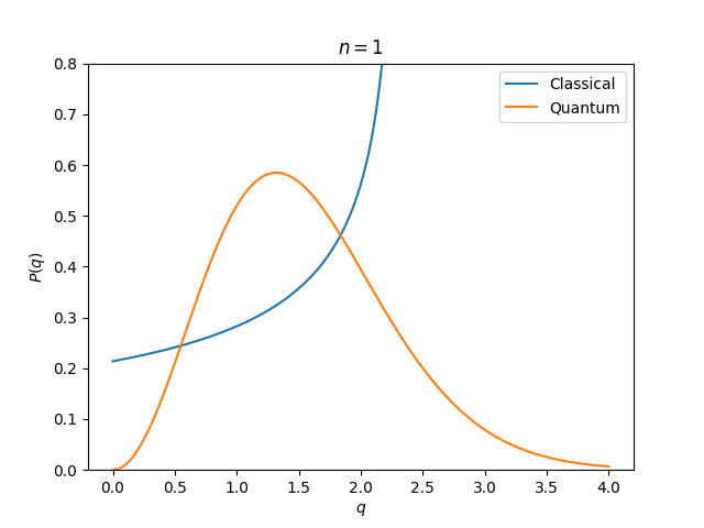
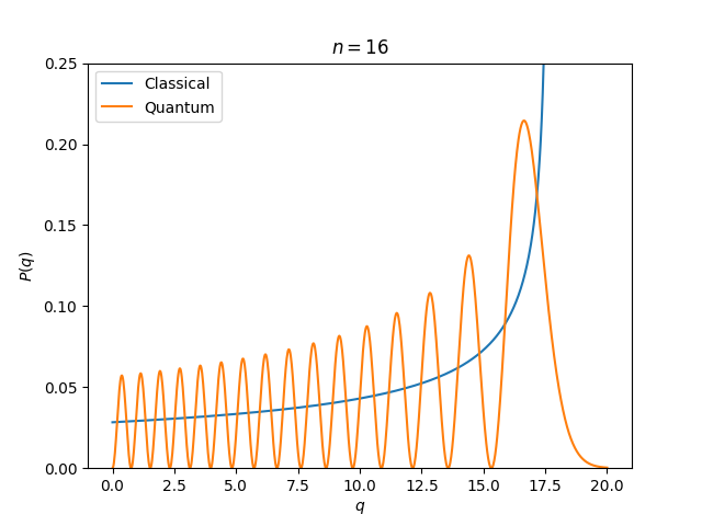
The following program plots the classical and quantum probability distributions, $P_\mathrm{cl}(z)$ and $|\psi(z)|^2$ , for $$n=1$$ and $$n=16$$ .

quantumairy

import numpy as np
from scipy.special import airy, ai_zeros
import matplotlib.pyplot as plt

nmax = 16

# Find the first nmax zeros of Ai(x)
a, _, _, _ = ai_zeros(nmax)
# The actual boundary condition is Ai(-qE) = 0 at q=0, so:
qE = -a


def prob_qm(n, dq):
    """
    Return the quantum mechanical probability density for a particle moving
    in a uniform gravitational field.

    """
    # The quantum mechanical wavefunction is proportional to Ai(q-qE) where
    # the qE corresponding to quantum number n is indexed at n-1
    psi, _, _, _ = airy(q - qE[n - 1])
    # Return the probability density, after rough-and-ready normalization
    P = psi**2
    return P / (sum(P) * dq)


def prob_cl(n):
    """
    Return the classical probability density for a particle bouncing
    elastically in a uniform gravitational field.

    """
    # The classical probability density is already normalized
    return 0.5 / np.sqrt(qE[n - 1] * (qE[n - 1] - q))


# The ground state, n=1
q, dq = np.linspace(0, 4, 1000, retstep=True)
plt.plot(q, prob_cl(1), label="Classical")
plt.plot(q, prob_qm(1, dq), label="Quantum")
plt.ylim(0, 0.8)
plt.xlabel("$q$")
plt.ylabel("$P(q)$")
plt.legend()
plt.title("$n=1$")
plt.show()

# An excited state, n=16
q, dq = np.linspace(0, 20, 1000, retstep=True)
plt.plot(q, prob_cl(16), label="Classical")
plt.plot(q, prob_qm(16, dq), label="Quantum")
plt.ylim(0, 0.25)
plt.xlabel("$q$")
plt.ylabel("$P(q)$")
plt.legend(loc="upper left")
plt.title("$n=16$")
plt.show()

We use scipy.special.ai_zeros to retrieve the $$n=1$$ and $$n=16$$ eigenvalues.
scipy.special.airy finds the corresponding wavefunctions and hence probability densities.
For the sake of illustration, these are normalized approximately by a very simple numerical integration.

Ground state of a particle in a gravitational field

The n=16 state of a particle in a gravitational field.

E8.2A quantum particle in a gravitational field